Table of Contents
Get source code for this RMarkdown script here.
Consider being a patron and supporting my work?
Donate and become a patron: If you find value in what I do and have learned something from my site, please consider becoming a patron. It takes me many hours to research, learn, and put together tutorials. Your support really matters.
# load libraries for analyses
library(data.table); library(lavaan)
Lord’s Paradox
Here’s a common study for scientific studies: Participants are randomly assigned to either receive a drug or a placebo (control condition). To evaluate the effects of the treatment (drug vs placebo control), you measure participants on some outcome measure before (pre-intervention) and after the intervention (post-intervention).
It seems like there are different ways to analyze the data and they sometimes can lead to different and even opposite results. This paradox is known as Lord’s Paradox because it was first reported by Frederic Lord (in 1967).

How can we analyze the data?
- Change-score approach: You can subtract the pre score from the post score
post - preand fit a model to this difference or change score. That is, a t-test or linear regression that compares change scores between the drug and control conditions.
- This difference/change-score model gives the total effect of condition (total effect: direct + indirect effects).
- Covariate approach: Or you can adjust for the effect of pre score (baseline) by including it as a covariate in your model. That is, you fit an ANCOVA or linear regression that models post score as a function of condition and post score (covariate).
- This covariate model gives you the direct effect of condition.
These two approaches often lead to different results, and is known as Lord’s Paradox. Judea Pearl(Pearl 2016) explains this paradox very well and has “resolved” this paradox by showing that both approaches are correct, but they uncover different effects or paths in the causal diagram.
Let’s play with fake data to understand this paradox.
Create fake data
Experimental design: 2 experimental conditions (drug vs control) (condition); 6 subjects (3 per condition) (id); measure of pre-experiment score (pre); measure of post-experiment score (post)
dt1 <- data.table(id = c(1, 2, 3, 4, 5, 6), # subject ids
           condition = factor(rep(c("drug", "control"), each = 3)), # between-subjects intervention
           pre = c(10, 20, 40, 20, 50, 30), # pre score (baseline)
           post = c(70, 60, 90, 10, 10, 20) # post score
           )
dt1[, change := post - pre]  # compute change score
dt1
   id condition pre post change
1:  1      drug  10   70     60
2:  2      drug  20   60     40
3:  3      drug  40   90     50
4:  4   control  20   10    -10
5:  5   control  50   10    -40
6:  6   control  30   20    -10
Mean change score for each condition:
dt1[, .(change_group_mean = mean(change)), by = condition]
   condition change_group_mean
1:      drug                50
2:   control               -20
Clearly the drug intervention is super effective.
Draw causal diagram
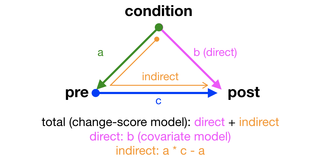
We can draw a directed acyclic graph (DAG) to represent our experimental design. DAGs are super useful for drawing inferences and making clear the paths and assumptions in our models and experimental designs. This figure is adapted from Pearl’s paper(Pearl 2016).
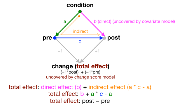
There are three path coefficients to be estimated in this DAG: a, b, and c.
c: the relationship (blue) betweenpreandpost, which can be estimated using the covariate approachb: is the direct effect (pink) of condition onpost, which can also be estimated using the covariate approacha: we don’t expect our intervention to affectpre, but it’s needed in the model to evaluate the indirect effect (orange) ofconditiononpost; think of it as the effect of drug/control treatment (condition) will have different effects on the outcome (post), depending on people’s baselines (pre)
Other effects that can be computed from these three coefficients:
total effect: direct (pink) + indirect effect (orange); which is also the change score that can be obtained using the change-score approach; also equivalent to+1 * post -1 * preindirect effect:
a * c - a, which captures the indirect effect ofconditiononpostwhile subtracting effect ofconditiononpre(i.e., patha)
Important observations
- If path
aorcis 0, then the indirect path ofconditiononpostviapremust be 0. Pathacan be 0 if we have perfect experimental control via perfect random assignment (which never happens in real life)—when participants in the two different experimental conditions have exactly the sameprescores. In that case, all effects ofconditionwill be direct (via pathb). You can change the fake data above to test the effects of the two conditions having the sameprescores.
Causal inference via structural equation model (SEM)
Define causal diagram using structural equation model syntax in lavaan package. The details of how to specify the DAG above in lavaan aren’t important here.
I specify two regression models (see comments in below). I’m telling lavaan to estimate three path coefficients for me a, b, and c, and then deterine other path coefficients (total, direct, indirect) based on these three coefficients.
model <-"
# regression 1
pre ~ a * condition
# a: lm(pre ~ condition) # condition effect

# regression 2
post ~ b * condition + c * pre
# b: lm(post ~ condition + pre, dt1) # condition effect on post (adjust for pre ;ANCOVA)
# c: lm(post ~ condition + pre, dt1) # pre effect on post (adjust for condition; ANCOVA)

# define parameters to understand DAG, covariate/change-score
total := b + a * c - a
# total: lm(change ~ condition, dt1) # condition effect on change score (total effect)
direct := b
indirect := a * c - a  # or total - direct
"
Fit the SEM or DAG using lavaan’s sem function
sem_results <- sem(model, dt1)Interpret model results
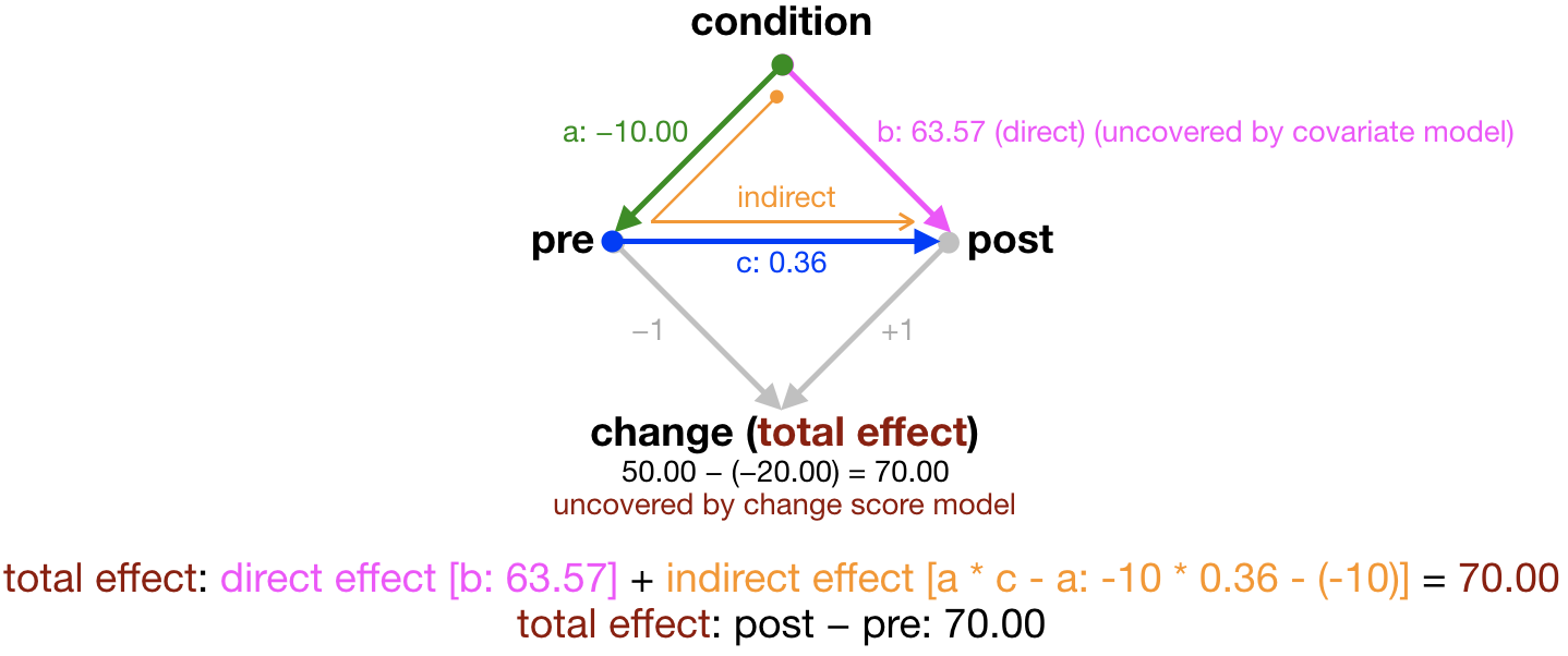
lavaan’s model output contains a lot of information that isn’t necessary for this tutorial, so I’ve summarized the main path coefficients we care about below.
    outcome    effect effect_label    est                       desc
1:      pre condition            a -10.00        lm(pre ~ condition)
2:     post condition            b  63.57 lm(post ~ condition + pre)
3:     post       pre            c   0.36 lm(post ~ condition + pre)
4:    total   b+a*c-a        total  70.00     lm(change ~ condition)
5:   direct         b       direct  63.57       same as line 2 above
6: indirect     a*c-a     indirect   6.43               total-direct
Rows 1 to 3 contain the estimated path coefficients a, b, c estimated using structural equation modeling (SEM). The last column desc tells you the regression model (e.g., covariate model or change-score model) to obtain that coefficient (which I’ll show below).
Note that the estimated total effect b + a * c - a is in fact the difference in mean change between the two conditions (70). The total effect, which is the difference in change score between the two conditions, is the sum of the direct and indirect effects.
Conclusion: The DAG and SEM contain all the information of covariate and change-score models!
Compare results with covariate and change-score models
Let’s fit the covariate model and change-score linear regression models to see how the results form these models map on to the results obtained using SEM.
Path a is the model we don’t typically fit. It captures the effect of condition on pre score.
path_a <- lm(pre ~ condition, dt1) # path a
round(coef(path_a)[-1], 2) # see row 1 of table above
conditiondrug
          -10
Paths b and c are captured by the covariate model. It captures the direct effect of condition on post score after adjusting for pre score (and also effect of pre on post after adjusting for condition).
paths_bc <- lm(post ~ condition + pre, dt1) # paths b (condition) and c (pre)
round(coef(paths_bc)[-1], 2) # see rows 2, 3, and 5 of table above
conditiondrug           pre
        63.57          0.36
The change-score model captures the total effect (the effect of condition on the change or difference score).
total <- lm(change ~ condition, dt1) # total effect (change score): b + a * c - a
round(coef(total)[-1], 2) # see row 4 of table above
conditiondrug
           70
Resources
If you want to learn more, read Pearl’s(Pearl 2016) paper and check out the resources below by Michael Clark.
Support my work
Support my work and become a patron here!
Pearl, Judea. 2016. “Lord’s Paradox Revisited – (Oh Lord! Kumbaya!).” Journal of Causal Inference 4 (2). http://dx.doi.org/10.1515/jci-2016-0021.