What happens when you set the intercept to 0 in regression models

What happens when you force the intercept to be 0 in a regression model and why you should (generally) never do it

Table of Contents

• Consider being a patron and supporting my work?
• Fit simple regression model (with intercept)
• Fit simple regression model without intercept
• Fit simple regression models with mean-centered regressor
• Additional resources
• Support my work

---

Get source code for this RMarkdown script here.

Consider being a patron and supporting my work?

Donate and become a patron: If you find value in what I do and have learned something from my site, please consider becoming a patron. It takes me many hours to research, learn, and put together tutorials. Your support really matters.

This article answers the questions below. I will use the built-in dataset mtcars.

• What is the intercept in a regression model?
• What happens when you remove or set the intercept to 0 in a regression model?
• Why you should never remove or set the intercept to 0?
• What are the effects of mean-centering a regressor/predictor?

If you need a refresher on how to interpret regression coefficients, see my other article.

library(ggplot2) # plot regression lines

Have a look at the built-in mtcars dataset.

head(mtcars)

                   mpg cyl disp  hp drat    wt  qsec vs am gear carb
Mazda RX4         21.0   6  160 110 3.90 2.620 16.46  0  1    4    4
Mazda RX4 Wag     21.0   6  160 110 3.90 2.875 17.02  0  1    4    4
Datsun 710        22.8   4  108  93 3.85 2.320 18.61  1  1    4    1
Hornet 4 Drive    21.4   6  258 110 3.08 3.215 19.44  1  0    3    1
Hornet Sportabout 18.7   8  360 175 3.15 3.440 17.02  0  0    3    2
Valiant           18.1   6  225 105 2.76 3.460 20.22  1  0    3    1

Fit simple regression model (with intercept)

model1 <- lm(mpg ~ disp, mtcars) # the intercept is included by default: lm(mpg ~ 1 + disp, mtcars)
coef1 <- coef(model1) # get coefficients
coef1

(Intercept)        disp 
29.59985476 -0.04121512 

Regression equation:

\[mpg_{i} = 29.59 - 0.04*disp_{i}\]

Interpretation

• For every 1 unit increase in the predictor disp, the outcome mpg changes by -0.04. That is, as disp increases, mpg decreases.
• When disp = 0, mpg = 29.59.

\[mpg = 29.59 - 0.04*0\]

\[mpg = 29.59\]

ggplot(mtcars, aes(disp, mpg)) +
  geom_point() +
  geom_vline(xintercept = 0, col = 'grey') +
  geom_hline(yintercept = 0, col = 'grey') +
  scale_x_continuous(limits = c(-10, max(mtcars$disp))) +
  scale_y_continuous(limits = c(-10, max(mtcars$mpg))) +
  geom_abline(intercept = coef(model1)[1], slope = coef(model1)[2]) # manually plot regression line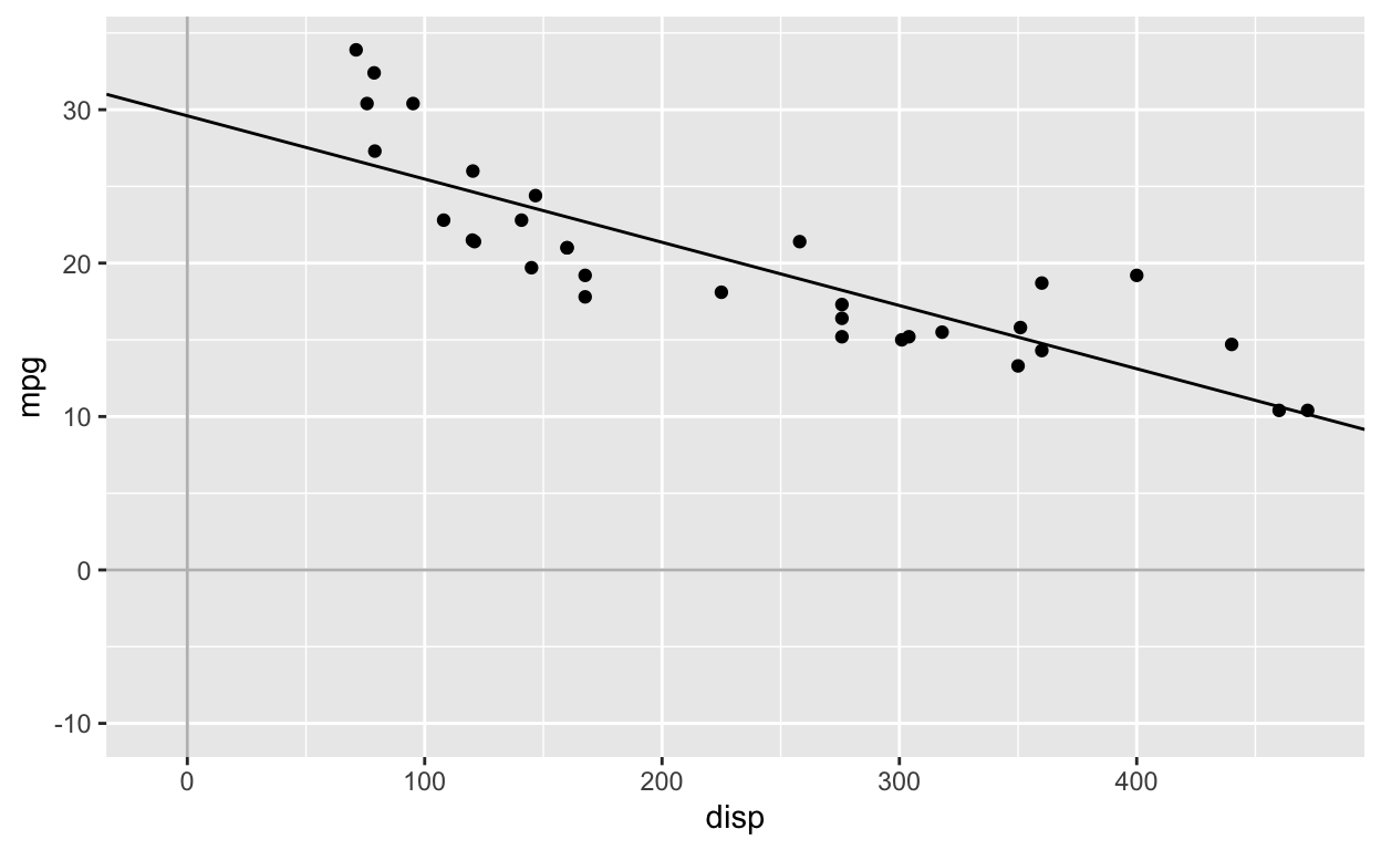

Fit simple regression model without intercept

model0 <- lm(mpg ~ 0 + disp, mtcars) # equivalent syntax: lm(mpg ~ -1 + disp, mtcars)
coef0 <- coef(model0) # get coefficients
coef0

      disp 
0.05904912 

Note that after setting the intercept to 0, the relationship between mpg and disp is now POSITIVE, rather than negative (see above model with intercept).

Regression equation:

\[mpg_{i} = 0 + 0.059*disp_{i}\]

Interpretation

• For every 1 unit increase in the predictor disp, the outcome mpg changes by 0.059. That is, as disp increases, mpg increases.
• When disp = 0, mpg = 0. By removing the intercept (i.e., setting it to 0), we are forcing the regression line to go through the origin (the point where disp = 0 and mpg = 0).

\[mpg = 0 + 0.059*0\]

\[mpg = 0\]

The regression line is forced to pass through the origin (0, 0). Therefore, unless your regressors are standardized or mean-centered, it’s not a good idea to set the intercept to 0 when fitting the model. Even when your regressors are standardized or mean-centered, you should still include the intercept.

ggplot(mtcars, aes(disp, mpg)) +
  geom_point() +
  geom_vline(xintercept = 0, col = 'grey') +
  geom_hline(yintercept = 0, col = 'grey') +
  scale_x_continuous(limits = c(-10, max(mtcars$disp))) +
  scale_y_continuous(limits = c(-10, max(mtcars$mpg))) +
  geom_abline(intercept = 0, slope = coef(model0)[1]) # manually plot regression line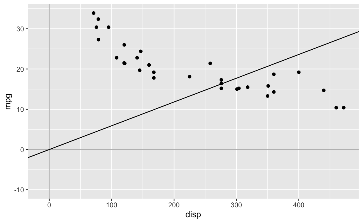

Fit simple regression models with mean-centered regressor

Mean-center regressor

mtcars$dispC <- mtcars$disp - mean(mtcars$disp) # create mean-centered variable
mean(mtcars$dispC) # mean of dispC is 0 (with some rounding error)

[1] -1.199041e-14

Fit model with intercept and mean-centered regressor

model1c <- lm(mpg ~ dispC, mtcars)
coef(model1c)

(Intercept)       dispC 
20.09062500 -0.04121512 

The intercept is now the the mean of outcome variable mpg. Check it by running mean(mtcars$mpg).

Fit model without intercept and with mean-centered regressor

model0c <- lm(mpg ~ 0 + dispC, mtcars)
coef(model0c)

      dispC 
-0.04121512 

After mean-centering the regressor/predictor, fitting the model with or without the intercept gives the same dispC coefficient: -0.04

ggplot(mtcars, aes(dispC, mpg)) +
  geom_point() +
  geom_vline(xintercept = 0, col = 'grey') +
  geom_hline(yintercept = 0, col = 'grey') +
  scale_x_continuous(limits = c(min(mtcars$dispC), max(mtcars$dispC))) +
  scale_y_continuous(limits = c(-10, max(mtcars$mpg))) +
  geom_abline(intercept = coef(model1c)[1], slope = coef(model1c)[2])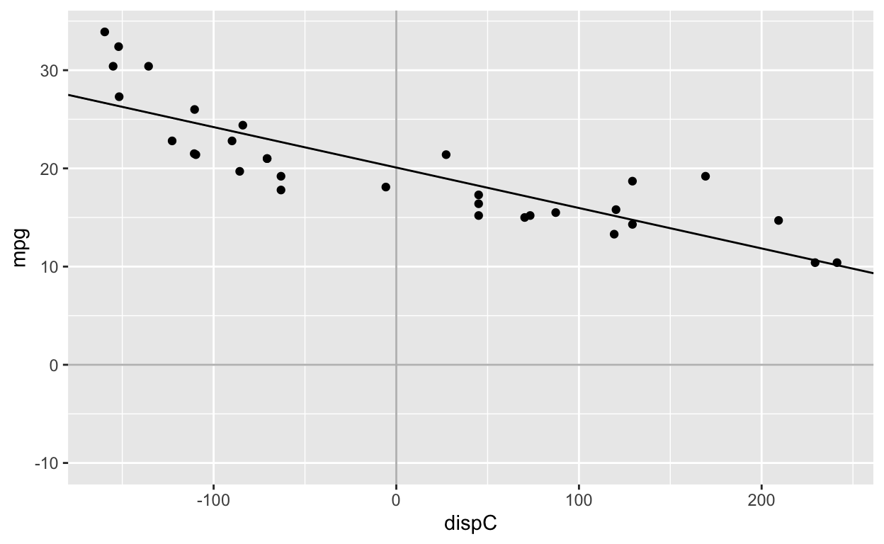 

Note that the regression slope is identical to the first figure. The only difference is that the points have been shifted to the left.

Additional resources

• StackExchange: When is it ok to remove the intercept in a linear regression model?

• Interpreting regression coefficients.

Support my work

Support my work and become a patron here!