Data science: Interpreting regression coefficients (including interaction coefficients)

Hause Lin

Get source code for this RMarkdown script here.

Consider being a patron and supporting my work?

Donate and become a patron: If you find value in what I do and have learned something from my site, please consider becoming a patron. It takes me many hours to research, learn, and put together tutorials. Your support really matters.

This tutorial provides a step-by-step introduction to interpreting regression coefficients in linear models. I will use the built-in dataset mtcars.

General guidelines for interpreting regression coefficients

intercept coefficient term (b0): the value of the outcome variable when all predictors = 0
all other non-interaction coefficients: the change in the outcome variable when the predictor increases by 1
interaction coefficients: the change in a coefficient value when one predictor increases by 1


library(data.table)  # to manipulate dataframes
library(interactions)  # to plot interactions later on
library(ggplot2)

Have a look at the mtcars dataset.


dt1 <- as.data.table(mtcars)  # convert to datatable
dt1


     mpg cyl  disp  hp drat    wt  qsec vs am gear carb
 1: 21.0   6 160.0 110 3.90 2.620 16.46  0  1    4    4
 2: 21.0   6 160.0 110 3.90 2.875 17.02  0  1    4    4
 3: 22.8   4 108.0  93 3.85 2.320 18.61  1  1    4    1
 4: 21.4   6 258.0 110 3.08 3.215 19.44  1  0    3    1
 5: 18.7   8 360.0 175 3.15 3.440 17.02  0  0    3    2
 6: 18.1   6 225.0 105 2.76 3.460 20.22  1  0    3    1
 7: 14.3   8 360.0 245 3.21 3.570 15.84  0  0    3    4
 8: 24.4   4 146.7  62 3.69 3.190 20.00  1  0    4    2
 9: 22.8   4 140.8  95 3.92 3.150 22.90  1  0    4    2
10: 19.2   6 167.6 123 3.92 3.440 18.30  1  0    4    4
11: 17.8   6 167.6 123 3.92 3.440 18.90  1  0    4    4
12: 16.4   8 275.8 180 3.07 4.070 17.40  0  0    3    3
13: 17.3   8 275.8 180 3.07 3.730 17.60  0  0    3    3
14: 15.2   8 275.8 180 3.07 3.780 18.00  0  0    3    3
15: 10.4   8 472.0 205 2.93 5.250 17.98  0  0    3    4
16: 10.4   8 460.0 215 3.00 5.424 17.82  0  0    3    4
17: 14.7   8 440.0 230 3.23 5.345 17.42  0  0    3    4
18: 32.4   4  78.7  66 4.08 2.200 19.47  1  1    4    1
19: 30.4   4  75.7  52 4.93 1.615 18.52  1  1    4    2
20: 33.9   4  71.1  65 4.22 1.835 19.90  1  1    4    1
21: 21.5   4 120.1  97 3.70 2.465 20.01  1  0    3    1
22: 15.5   8 318.0 150 2.76 3.520 16.87  0  0    3    2
23: 15.2   8 304.0 150 3.15 3.435 17.30  0  0    3    2
24: 13.3   8 350.0 245 3.73 3.840 15.41  0  0    3    4
25: 19.2   8 400.0 175 3.08 3.845 17.05  0  0    3    2
26: 27.3   4  79.0  66 4.08 1.935 18.90  1  1    4    1
27: 26.0   4 120.3  91 4.43 2.140 16.70  0  1    5    2
28: 30.4   4  95.1 113 3.77 1.513 16.90  1  1    5    2
29: 15.8   8 351.0 264 4.22 3.170 14.50  0  1    5    4
30: 19.7   6 145.0 175 3.62 2.770 15.50  0  1    5    6
31: 15.0   8 301.0 335 3.54 3.570 14.60  0  1    5    8
32: 21.4   4 121.0 109 4.11 2.780 18.60  1  1    4    2
     mpg cyl  disp  hp drat    wt  qsec vs am gear carb

Linear regression with one continuous predictor


head(dt1)  # check data


    mpg cyl disp  hp drat    wt  qsec vs am gear carb
1: 21.0   6  160 110 3.90 2.620 16.46  0  1    4    4
2: 21.0   6  160 110 3.90 2.875 17.02  0  1    4    4
3: 22.8   4  108  93 3.85 2.320 18.61  1  1    4    1
4: 21.4   6  258 110 3.08 3.215 19.44  1  0    3    1
5: 18.7   8  360 175 3.15 3.440 17.02  0  0    3    2
6: 18.1   6  225 105 2.76 3.460 20.22  1  0    3    1


model_continuous_predictor <- lm(mpg ~ wt, dt1)
# summary(model_continuous_predictor)
coef(model_continuous_predictor)


(Intercept)          wt 
  37.285126   -5.344472

-5.34: whenever wt increases by 1 (unit), mpg changes by this amount
37.29: whenever wt is 0, mpg is this value (i.e., intercept: the value of mpg when wt = 0, of the value of the outcome variable when the predictor is 0)

Note that in the data, wt only takes on values between 1 and 5, so the intercept of 37.29 is an extrapolation of the regression line to wt values that don’t exist in our data (see figure below).


ggplot(dt1, aes(wt, mpg)) +
  geom_vline(xintercept = 0) +
  geom_point() +
  geom_smooth(method = 'lm', formula = y ~ poly(x, 1), fullrange = TRUE) +
  scale_x_continuous(limits = c(-1, 7), breaks = -1:7) +
  annotate("text", x = 1.7, y = coef(model_continuous_predictor)[1] + 2,
           label = paste0(round(coef(model_continuous_predictor)[1], 2), " (intercept)"),
           size = 6)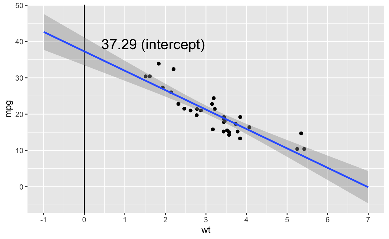

Linear regression with one categorical predictor (two levels)


head(dt1)  # check data (vs is a binary variable with just 0 and 1)


    mpg cyl disp  hp drat    wt  qsec vs am gear carb
1: 21.0   6  160 110 3.90 2.620 16.46  0  1    4    4
2: 21.0   6  160 110 3.90 2.875 17.02  0  1    4    4
3: 22.8   4  108  93 3.85 2.320 18.61  1  1    4    1
4: 21.4   6  258 110 3.08 3.215 19.44  1  0    3    1
5: 18.7   8  360 175 3.15 3.440 17.02  0  0    3    2
6: 18.1   6  225 105 2.76 3.460 20.22  1  0    3    1


dt1[, vs_factor := as.factor(vs)]  # turn vs into a factor
model_categorical_predictor <- lm(mpg ~ vs_factor, dt1)
# summary(model_categorical_predictor)
coef(model_categorical_predictor)


(Intercept)  vs_factor1 
  16.616667    7.940476

When the categorical predictor has only two levels (coded 0 and 1), we can use the numeric variable as the predictor. We’ll get the same results as above.


coef(lm(mpg ~ vs_factor, dt1))  # factor predictor


(Intercept)  vs_factor1 
  16.616667    7.940476


coef(lm(mpg ~ vs, dt1))  # numeric predictor


(Intercept)          vs 
  16.616667    7.940476

7.94: whenever vs_factor increases by 1 (unit), mpg changes by this amount; here, when vs = 0 is one categorical level/condition, and vs = 1 is the second categorical level/condition; thus this value refers to the difference in mean values between the two conditions
16.62: whenever vs_factor is 0, mpg is this value (i.e., intercept: the value of y when x = 0); thus, the intercept is the mean of the values when vs = 0.

The vs_factor coefficient name has a 1 at the end (vs_factor1). Why? R has coded the intercept as vs = 0 (i.e., vs_factor0) and vs = 1 as the next level (i.e., vs_factor1). Hence the coefficient in this model is the difference between the means of the two levels.

To show you the interpretation of the coefficients is indeed correct, let’s manually compute the mean of the two conditions (vs = 0, vs = 1) and compute their difference.


# compute mean mpg for each vs condition
vs_condition_means <- dt1[, .(mpg_group_mean = mean(mpg)), keyby = vs]
vs_condition_means


   vs mpg_group_mean
1:  0       16.61667
2:  1       24.55714

The mean mpg value for the group vs = 0 is the same as the intercept value from the regression above (16.62).


# compute difference in mpg value between vs conditions
vs_condition_means$mpg_group_mean[2] - vs_condition_means$mpg_group_mean[1]


[1] 7.940476

The difference in mean mpg values between the two vs conditions is the same as the slope (beta coefficient) from the regression above (7.94).


ggplot(dt1, aes(vs, mpg)) +
  geom_point() +
  geom_smooth(method = 'lm', formula = y ~ poly(x, 1), fullrange = TRUE)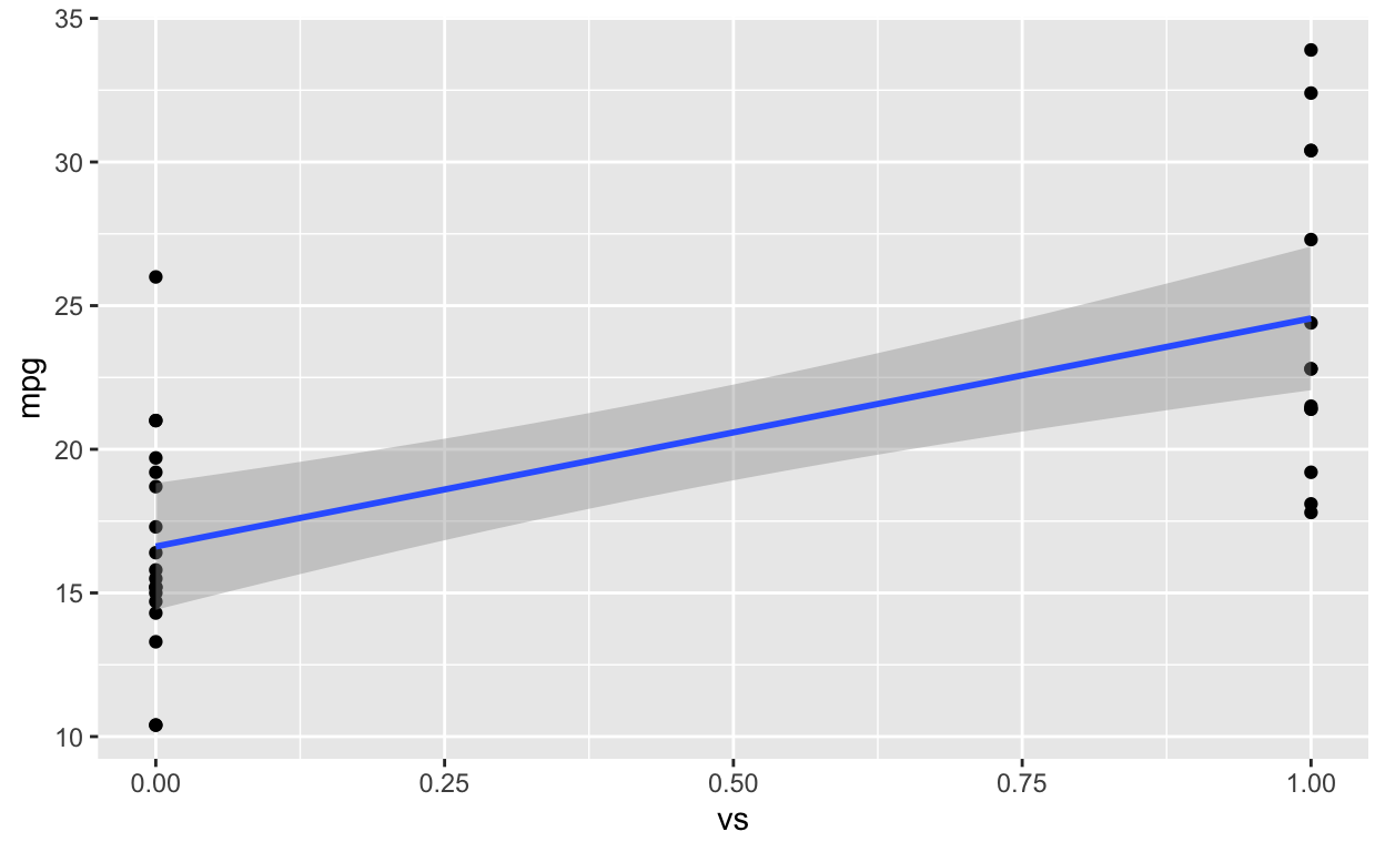

Linear regression with one categorial predictor (three levels)


head(dt1)  # check data (cyl is a categorical predictor with 3 levels)


    mpg cyl disp  hp drat    wt  qsec vs am gear carb vs_factor
1: 21.0   6  160 110 3.90 2.620 16.46  0  1    4    4         0
2: 21.0   6  160 110 3.90 2.875 17.02  0  1    4    4         0
3: 22.8   4  108  93 3.85 2.320 18.61  1  1    4    1         1
4: 21.4   6  258 110 3.08 3.215 19.44  1  0    3    1         1
5: 18.7   8  360 175 3.15 3.440 17.02  0  0    3    2         0
6: 18.1   6  225 105 2.76 3.460 20.22  1  0    3    1         1


dt1[, cyl_factor := as.factor(cyl)]  # turn cyl into a factor
model_categorical_predictor_3 <- lm(mpg ~ cyl_factor, dt1)
# summary(model_categorical_predictor_3)
coef(model_categorical_predictor_3)


(Intercept) cyl_factor6 cyl_factor8 
  26.663636   -6.920779  -11.563636

When the categorical predictor has three or more levels, we can’t use the numeric variable as the predictor because the coefficients will be different.


coef(lm(mpg ~ cyl, dt1))  # numeric predictor


(Intercept)         cyl 
   37.88458    -2.87579


coef(lm(mpg ~ cyl_factor, dt1))  # factor predictor


(Intercept) cyl_factor6 cyl_factor8 
  26.663636   -6.920779  -11.563636

Interpreting the coefficients in the model with the categorical predictor

When we convert variables to factors or characters, R automatically represents the “smallest” condition (1 is smaller than 9; “a” is smaller than “b”) as the intercept. In other words, this condition is treated assigned the value 0 and all other conditions are assigned 1. That is, R by default uses “dummy coding”.
26.66: when cyl_factor is 4 (or the “smallest” cyl_factor value in the dataset), mpg is this value (i.e., intercept); thus, the intercept is the mean of the values when cyl_factor = 4.
-6.92: difference in mean mpg values between the conditions cyl_factor = 4 and cyl_factor = 6
-11.56: difference in mean mpg values between the conditions cyl_factor = 4 and cyl_factor = 8

To show you the interpretation of the coefficients is indeed correct, let’s manually compute the mean of the three conditions (cyl_factor is 4, 6, 8) and compute their differences.


# compute mean mpg for each vs condition
cyl_condition_means <- dt1[, .(mpg_group_mean = mean(mpg)), keyby = cyl_factor]
cyl_condition_means


   cyl_factor mpg_group_mean
1:          4       26.66364
2:          6       19.74286
3:          8       15.10000

The mean mpg value for the group cyl_factor = 4 is the same as the intercept value from the regression above.


# compute difference in mpg value between cyl = 6 and cyl = 4
cyl_condition_means$mpg_group_mean[2] - cyl_condition_means$mpg_group_mean[1]


[1] -6.920779


coef(model_categorical_predictor_3)[2]  # beta coefficient


cyl_factor6 
  -6.920779


# compute difference in mpg value between cyl = 8 and cyl = 4
cyl_condition_means$mpg_group_mean[3] - cyl_condition_means$mpg_group_mean[1]


[1] -11.56364


coef(model_categorical_predictor_3)[3]  # beta coefficient


cyl_factor8 
  -11.56364


ggplot(dt1, aes(cyl, mpg)) +
  geom_point() +
  geom_smooth(method = 'lm', formula = y ~ poly(x, 1), fullrange = TRUE)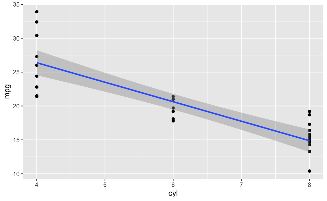

When fitting the regression model, R uses dummy coding by default. Hence, the condition cyl = 4 is actually assigned 0 (and thus is the intercept).

Linear regression with continuous predictor, categorical predictor (two levels), and their interaction

Let’s fit a regression model that includes an interaction term.


model_interaction1 <- lm(mpg ~ disp * vs_factor, data = dt1)
coef(model_interaction1)


    (Intercept)            disp      vs_factor1 disp:vs_factor1 
    25.63755459     -0.02936965      8.39770888     -0.04218648

How do we interpret the interaction coefficient?

For every 1 unit increase in vs_factor (coded 0 and 1), the coefficient of disp changes by -0.042. READ THAT SENTENCE AGAIN TO SLOWLY DIGEST IT! It’s the change in the COEFFICIENT of disp when vs_factor increases by 1 (unit).

Let’s fit separate models for the two vs_factor conditions to verify the statement/interpretation above.

Fit linear models (mpg ~ disp) separately for vs_factor = 0 and vs_factor = 1.


model_mpg_disp_vs0 <- lm(mpg ~ disp, data = dt1[vs_factor == 0])  # blue line in figure below
model_mpg_disp_vs1 <- lm(mpg ~ disp, data = dt1[vs_factor == 1])  # orange line in figure below

Check the coefficeints of disp for these two models


coef(model_mpg_disp_vs0)


(Intercept)        disp 
25.63755459 -0.02936965


coef(model_mpg_disp_vs1)


(Intercept)        disp 
34.03526346 -0.07155613

Here’s a reminder (again) of how to interpret the disp * vs_factor interaction coefficient in the interaction model (mpg ~ disp * vs_factor): For every 1 unit increase in vs_factor (coded 0 and 1), the coefficient of disp changes by -0.042. Or the change in the COEFFICIENT of disp when vs_factor increases by 1 (unit).

Let’s compute the difference of the disp coefficients in the two models above (where vs is 0 and 1).


coef(model_mpg_disp_vs1)['disp'] - coef(model_mpg_disp_vs0)['disp']


       disp 
-0.04218648

The difference in the disp coefficients (-0.042) in the two models (where vs_factor is 1 or 0) is identical to the interaction coefficient (disp * factor: -0.042) in the model_interaction1 model.

In other words, the interaction coefficient is the difference between the values of the two slopes (i.e., coefficients) (see figure below).

mpg ~ disp when vs_factor = 0: disp coefficient is -0.029
mpg ~ disp when vs_factor = 1: disp coefficient is -0.072
The slope (i.e., coefficient) of disp in the mpg ~ disp model is more negative (by disp * factor: -0.042) when vs_factor = 1 than when vs_factor = 0.


interact_plot(model_interaction1, pred = disp, modx = vs_factor)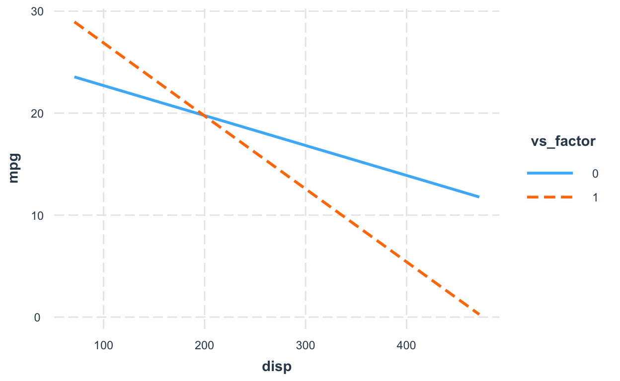

Linear regression with two continuous predictors and their interaction

You can interpret the interaction coefficients in all models (continuous or categorical variables) the same way.


model_interaction2 <- lm(mpg ~ disp * wt, data = dt1)  # all continuous predictors
coef(model_interaction2)


(Intercept)        disp          wt     disp:wt 
44.08199770 -0.05635816 -6.49567966  0.01170542

disp:wt = 0.012: the change in the coefficient of disp when wt increases by 1 unit (or the reverse is also fine: the change in the coefficient of wt when disp increases by 1 unit)

When all predictors are continuous variables, the convention is to plot the effect of one regressor at different levels (+/- 1 SD and mean value) of the other regressor.


interact_plot(model_interaction2, pred = wt, modx = disp)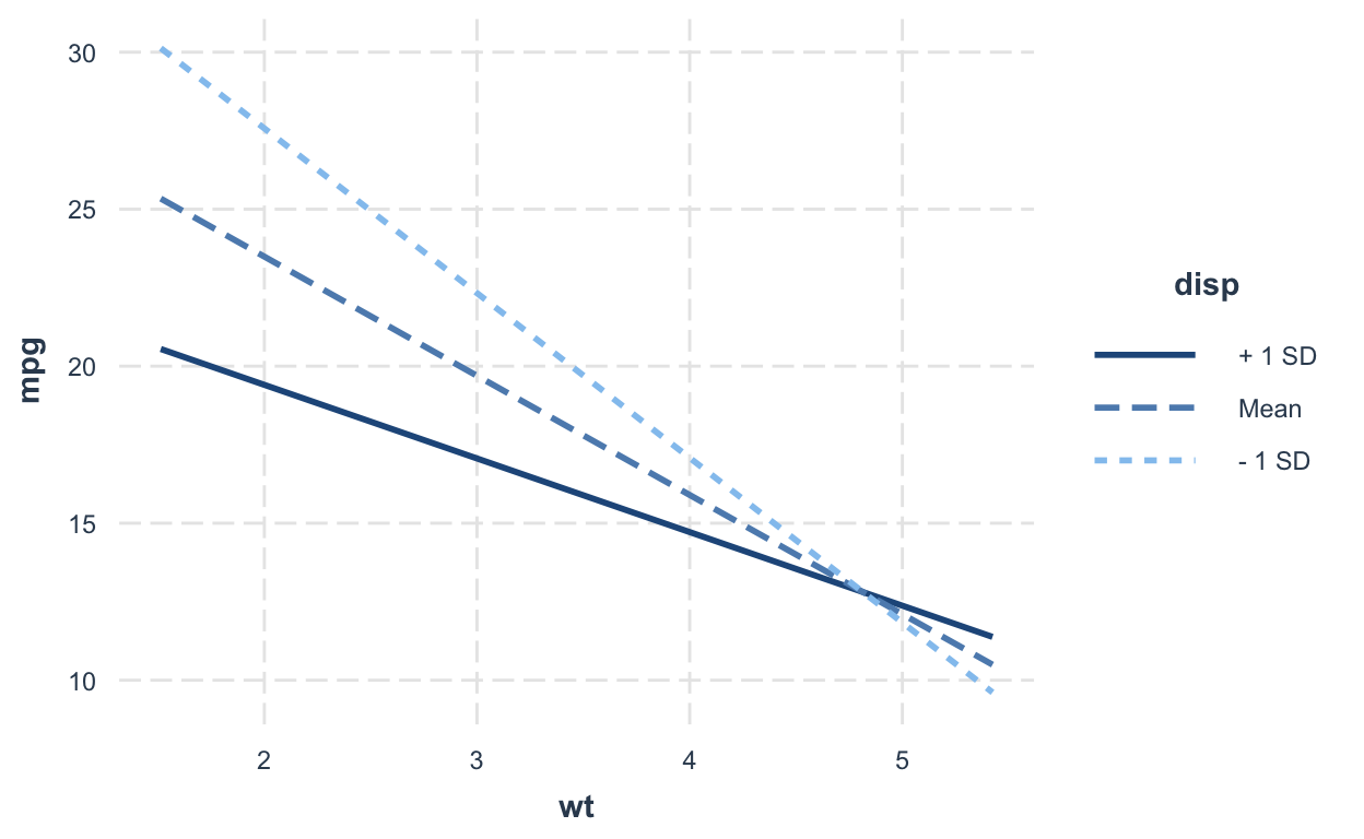


interact_plot(model_interaction2, pred = disp, modx = wt)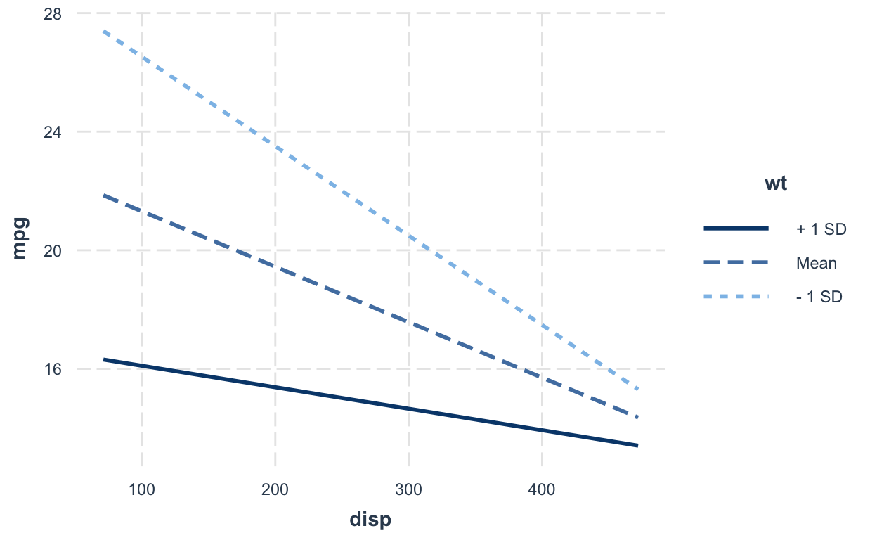

Linear regression with three- or four-way interactions

No matter how complicated your interaction terms are (3 or 4 or 10-way interactions), you interpret the coefficients the same way!


model_interaction4 <- lm(mpg ~ disp * wt * qsec * drat, data = dt1)  # all continuous predictors
coef(model_interaction4)["disp:wt:qsec:drat"]  # the 4-way interaction


disp:wt:qsec:drat 
        0.0301177

There are many ways to interpret the coefficient disp:wt:qsec:drat = 0.03:

when disp increases by 1, the wt:qsec:drat coefficient (slope) changes by 0.03
when wt increases by 1, the disp:qsec:drat coefficient (slope) changes by 0.03
when qsec increases by 1, the disp:wt:drat coefficient (slope) changes by 0.03
when drat increases by 1, the disp:wt:qsec coefficient (slope) changes by 0.03

You can also interpret the three- or two-way interactions in the same model in the same way. You get it…

Support my work

Support my work and become a patron here!

Comment on this article Share:

Interpreting regression coefficients (including interaction coefficients)

Table of Contents