Table of Contents
This tutorial shows you how to analyze simple reaction time and acccuracy data that resemble data collected from standard psychology experiments (note that the three subjects’ data were actually simulated with the rwiener function from the RWiener package). This package also assumes you know how to set your working directory; if not, check out my intro tutorials here.
I use the data.table package extensively in my analyses. tidyverse and dplyr are great, but I prefer the speed and concise syntax of data.table. I won’t explain how data.table works in this tutorial, but you’ll see in the code below how flexible and concise it is. If you want to learn more, see my tutorials and extra resources.
Consider being a patron and supporting my work?
Donate and become a patron: If you find value in what I do and have learned something from my site, please consider becoming a patron. It takes me many hours to research, learn, and put together tutorials. Your support really matters.
Getting the data and code
- Download Rmarkdown script for this tutorial here.
- Download data for all my tutorials here.
- Inside the data folder, you should see a
rt_acc_data_rawfolder that contains three subjects’ data, which we will analyze in this tutorial. - Leave the folders and files in the unzipped folder as they are because we’ll use R to read the csv files into our R environment.
Dataset information
- 3 subjects: 30, 35, 39
- Completed a task where reaction time (rt) and accuracy (acc) were collected
- 2 blocks in the experiment (1, 2)
- 40 trials per block; 4 blocks in total; 80 trials in total
- 2 experimental manipulations: reward available on trial (high vs low); instructions for block (focus on responding carefully [caution] vs focusing on responding quickly (speed))
Variables
- subject: subject id
- completed: whether subject completed study (1, 0)
- rt: reaction time
- acc: accuracy
- reward: reward available on trial (high or low)
- instructions: block instructions (caution or speed)
- block: block number (1, 2)
- trialinblock: trial in block (1 to 4 0)
- overalltrial: overall trial number (1 to 80)
Organizing folders/directory
This is how my directories/folders/files look like. You should make sure yours look similar before you continue.
— 0005_analyze_multi_subject_trial_data.Rmd
——— data
————— rt_acc_data_raw
——————— subject_30.csv
——————— subject_35.csv
——————— subject_39.csv
Load libraries
library(tidyverse); library(data.table); library(lme4); library(lmerTest); library(ggbeeswarm); library(hausekeep)Read all subjects’ data into R
(files <- list.files(path = "./data/rt_acc_data_raw", pattern = "subject_", full.names = TRUE)) # find matching file names
[1] "./data/rt_acc_data_raw/subject_30.csv"
[2] "./data/rt_acc_data_raw/subject_35.csv"
[3] "./data/rt_acc_data_raw/subject_39.csv"
dt1 <- bind_rows(lapply(files, fread)) %>% as.data.table() # read data, combine items in list, convert to data.tableNote and explanation: lapply loops through each item in files and applies the fread function to each item. bind_rows combines all the dataframes stored as separate items in the list, and as.data.table() converts the merged dataframe into data.table class.
Summarize experimental design
dt1[, .N, by = subject] # rows (trials) per subject
   subject  N
1:      30 80
2:      35 80
3:      39 80
dt1[, .N, keyby = .(subject, block)] # blocks per subject and rows/trials per block
   subject block  N
1:      30     1 40
2:      30     2 40
3:      35     1 40
4:      35     2 40
5:      39     1 40
6:      39     2 40
dt1[, .N, keyby = .(subject, instructions, reward)] # row (trials) per subject for instructions/reward conditions
    subject instructions reward  N
 1:      30      caution   high 20
 2:      30      caution    low 20
 3:      30        speed   high 20
 4:      30        speed    low 20
 5:      35      caution   high 20
 6:      35      caution    low 20
 7:      35        speed   high 20
 8:      35        speed    low 20
 9:      39      caution   high 20
10:      39      caution    low 20
11:      39        speed   high 20
12:      39        speed    low 20
Remove outlier trials
dt1[rt < 0.2, `:=` (rt = NA, acc = NA)] # if rt < 0.2, convert rt and acc to NA (too fast response on that trial)
dt1[rt > 3.0, `:=` (rt = NA, acc = NA)] # if rt > 3.0, convert rt and acc to NA (too slow response on that trial)
summary(dt1$rt) # check range and number of NA
   Min. 1st Qu.  Median    Mean 3rd Qu.    Max.    NA's
 0.3573  0.6123  0.7982  0.9581  1.1328  2.8346      26
summary(dt1$acc) # check range and number of NA
   Min. 1st Qu.  Median    Mean 3rd Qu.    Max.    NA's
 0.0000  0.0000  1.0000  0.6869  1.0000  1.0000      26
Compute mean RT and ACC for each subject, for each condition
dt1_avg <- dt1[, .(rt = mean(rt, na.rm = T), acc = mean(acc, na.rm = T)), keyby = .(subject, instructions, reward)]
dt1_avg
    subject instructions reward        rt       acc
 1:      30      caution   high 1.2225593 0.8333333
 2:      30      caution    low 1.2616149 0.7222222
 3:      30        speed   high 0.7903719 0.7777778
 4:      30        speed    low 0.6023415 0.7222222
 5:      35      caution   high 1.1598959 0.8000000
 6:      35      caution    low 1.2455745 0.6111111
 7:      35        speed   high 0.7732939 0.6000000
 8:      35        speed    low 0.7355426 0.3333333
 9:      39      caution   high 1.2379130 0.9444444
10:      39      caution    low 1.0858297 0.5294118
11:      39        speed   high 0.7753915 0.7647059
12:      39        speed    low 0.6738280 0.6315789
Compute grand average RT and ACC (and within-subject error bars)
dt1_grdavg <- seWithin(data = dt1_avg, measurevar = c("rt", "acc"), withinvars = c("instructions", "reward"), idvar = "subject")
Confidence intervals: 0.95Confidence intervals: 0.95$rt
   instructions reward N        rt         sd         se        ci
1:      caution   high 3 1.2067894 0.06623893 0.03824307 0.1645466
2:      caution    low 3 1.1976730 0.09257261 0.05344682 0.2299631
3:        speed   high 3 0.7796858 0.02221612 0.01282648 0.0551879
4:        speed    low 3 0.6705707 0.07532700 0.04349006 0.1871226

$acc
   instructions reward N       acc         sd         se         ci
1:      caution   high 3 0.8592593 0.10091676 0.05826432 0.25069114
2:      caution    low 3 0.6209150 0.12588855 0.07268179 0.31272449
3:        speed   high 3 0.7141612 0.02218782 0.01281015 0.05511761
4: speed low 3 0.5623782 0.12854647 0.07421634 0.31932713Plot reaction time
plot_rt <- ggplot(dt1_grdavg$rt, aes(instructions, rt, col = reward)) +
  geom_quasirandom(data = dt1_avg, alpha = 0.8, dodge = 1, size = 1.5) +
  geom_point(position = position_dodge(1), shape = 95, size = 6) +
  geom_errorbar(aes(ymin = rt - ci, ymax = rt + ci), position = position_dodge(1), width = 0, size = 1.1) +
  labs(y = "reaction time (95% CI)")
plot_rt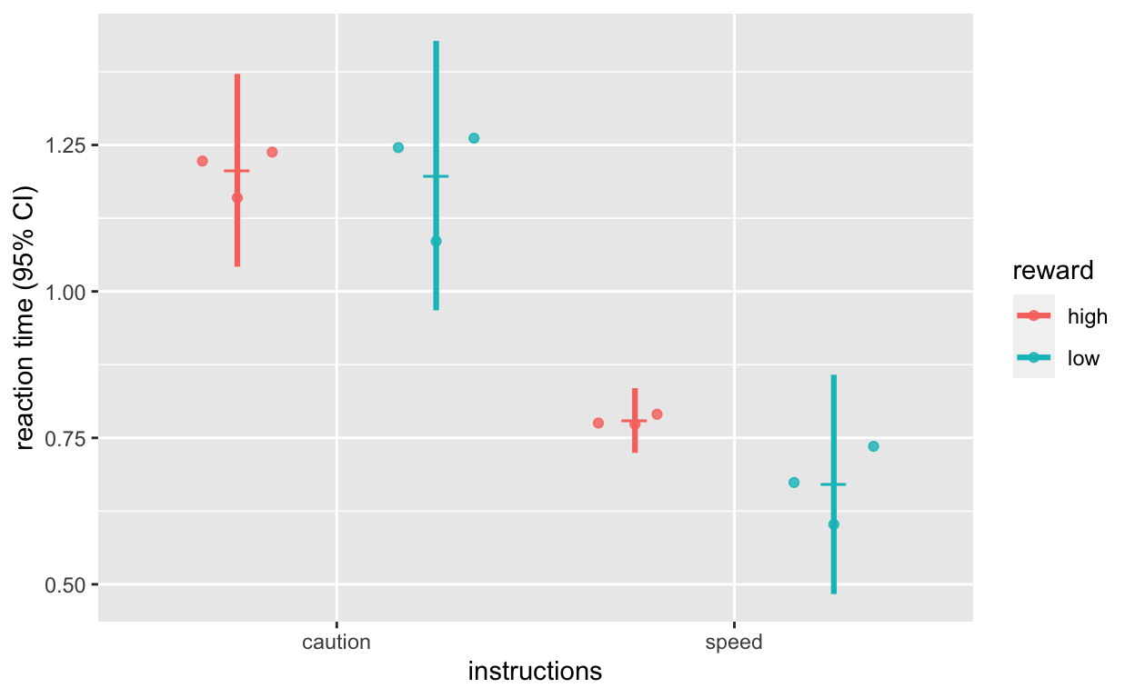
Plot accuracy
plot_acc <- ggplot(dt1_grdavg$acc, aes(instructions, acc, col = reward)) +
  geom_quasirandom(data = dt1_avg, alpha = 0.8, dodge = 1, size = 1.5) +
  geom_point(position = position_dodge(1), shape = 95, size = 6) +
  geom_errorbar(aes(ymin = acc - ci, ymax = acc + ci), position = position_dodge(1), width = 0, size = 1.1) +
  scale_y_continuous(limits = c(0, 1.2), breaks = seq(0, 1.0, 0.25)) +
  labs(y = "accuracy (95% CI)")
plot_acc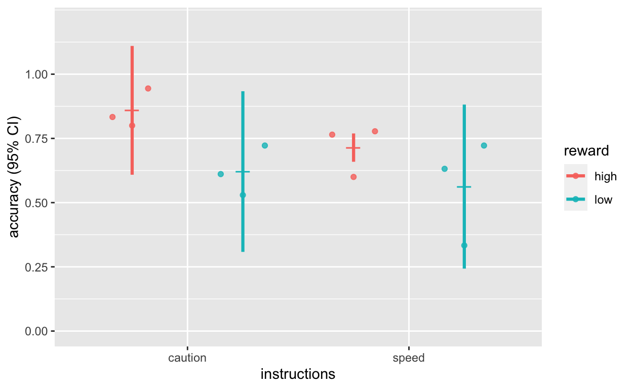
Fit linear mixed models to single-trial RT and ACC
model_rt <- lmer(rt ~ instructions + reward + (1 | subject), data = dt1)
summary(model_rt)
Linear mixed model fit by REML. t-tests use Satterthwaite's method [
lmerModLmerTest]
Formula: rt ~ instructions + reward + (1 | subject)
   Data: dt1

REML criterion at convergence: 276.1

Scaled residuals:
    Min      1Q  Median      3Q     Max
-1.8528 -0.6872 -0.2444  0.4666  3.6802

Random effects:
 Groups   Name        Variance Std.Dev.
 subject  (Intercept) 0.0000   0.000
 Residual             0.2034   0.451
Number of obs: 214, groups:  subject, 3

Fixed effects:
                   Estimate Std. Error        df t value Pr(>|t|)
(Intercept)         1.23552    0.05425 211.00000  22.774  < 2e-16 ***
instructionsspeed  -0.48007    0.06169 211.00000  -7.782 3.13e-13 ***
rewardlow          -0.06073    0.06167 211.00000  -0.985    0.326
---
Signif. codes:  0 '***' 0.001 '**' 0.01 '*' 0.05 '.' 0.1 ' ' 1

Correlation of Fixed Effects:
            (Intr) instrc
instrctnssp -0.590
rewardlow   -0.579  0.010
convergence code: 0
boundary (singular) fit: see ?isSingular
summaryh(model_rt) # summary function from my hausekeep package
                term                                                  results
1:       (Intercept)  b = 1.24, SE = 0.05, t(211) = 22.77, p < .001, r = 0.84
2: instructionsspeed b = −0.48, SE = 0.06, t(211) = −7.78, p < .001, r = 0.47
3:         rewardlow b = −0.06, SE = 0.06, t(211) = −0.98, p = .326, r = 0.07
model_acc <- glmer(acc ~ instructions + reward + (1 | subject), data = dt1, family = binomial)
summary(model_acc)
Generalized linear mixed model fit by maximum likelihood (Laplace
  Approximation) [glmerMod]
 Family: binomial  ( logit )
Formula: acc ~ instructions + reward + (1 | subject)
   Data: dt1

     AIC      BIC   logLik deviance df.resid
   260.9    274.3   -126.4    252.9      210

Scaled residuals:
    Min      1Q  Median      3Q     Max
-2.4415 -1.1104  0.5184  0.6717  1.0753

Random effects:
 Groups  Name        Variance Std.Dev.
 subject (Intercept) 0.0771   0.2777
Number of obs: 214, groups:  subject, 3

Fixed effects:
                  Estimate Std. Error z value Pr(>|z|)
(Intercept)         1.5925     0.3420   4.657 3.21e-06 ***
instructionsspeed  -0.5182     0.3083  -1.681  0.09283 .
rewardlow          -0.9411     0.3118  -3.018  0.00255 **
---
Signif. codes:  0 '***' 0.001 '**' 0.01 '*' 0.05 '.' 0.1 ' ' 1

Correlation of Fixed Effects:
            (Intr) instrc
instrctnssp -0.536
rewardlow   -0.571  0.061
summaryh(model_acc) # summary function from my hausekeep package
                term                                                   results
1:       (Intercept)    b = 1.59, SE = 0.34, z(210) = 4.66, p < .001, r = 0.40
2: instructionsspeed b = −0.52, SE = 0.31, z(210) = −1.68, p = .093, r = −0.14
3:         rewardlow b = −0.94, SE = 0.31, z(210) = −3.02, p = .003, r = −0.25