Table of Contents
Get source code for this RMarkdown script here.
Consider being a patron and supporting my work?
Donate and become a patron: If you find value in what I do and have learned something from my site, please consider becoming a patron. It takes me many hours to research, learn, and put together tutorials. Your support really matters.
Load packages/libraries
Use library() to load packages at the top of each R script.
library(tidyverse); library(data.table)Wide vs. long data (messy vs. tidy data)
Manually create wide data
wide <- tibble(student = c("Andy", "Mary"),
               englishGrades = c(1, -2),
               mathGrades = englishGrades * 10,
               physicsGrades = mathGrades * 100)
wide
# A tibble: 2 x 4
  student englishGrades mathGrades physicsGrades
  <chr>           <dbl>      <dbl>         <dbl>
1 Andy                1         10          1000
2 Mary -2 -20 -2000Manually create equivalent long data
long <- tibble(student = rep(c("Andy", "Mary"), each = 3),
               class = rep(c("englishGrades", "mathGrades", "physicsGrades"), times = 2),
               grades = c(1, 10, 1000, -2, -20, -2000))
long
# A tibble: 6 x 3
  student class         grades
  <chr>   <chr>          <dbl>
1 Andy    englishGrades      1
2 Andy    mathGrades        10
3 Andy    physicsGrades   1000
4 Mary    englishGrades     -2
5 Mary    mathGrades       -20
6 Mary    physicsGrades  -2000
Compare wide vs long data (“messy” vs. “tidy” data)
wide # wide/messy
# A tibble: 2 x 4
  student englishGrades mathGrades physicsGrades
  <chr>           <dbl>      <dbl>         <dbl>
1 Andy                1         10          1000
2 Mary               -2        -20         -2000
long # long/tidy
# A tibble: 6 x 3
  student class         grades
  <chr>   <chr>          <dbl>
1 Andy    englishGrades      1
2 Andy    mathGrades        10
3 Andy    physicsGrades   1000
4 Mary    englishGrades     -2
5 Mary    mathGrades       -20
6 Mary physicsGrades -2000Wide to long with melt() (from data.table)
There is a base R melt() function that is less powerful and slower than the melt() that comes with data.table. As long as you’ve loaded data.table with library(data.table), you’ll be using the more powerful version of melt().
melt(wide, id.vars = c("student"))
  student      variable value
1    Andy englishGrades     1
2    Mary englishGrades    -2
3    Andy    mathGrades    10
4    Mary    mathGrades   -20
5    Andy physicsGrades  1000
6    Mary physicsGrades -2000
Rename variables
melt(wide, id.vars = c("student"), variable.name = "cLaSs", value.name = "gRaDeS")
  student         cLaSs gRaDeS
1    Andy englishGrades      1
2    Mary englishGrades     -2
3    Andy    mathGrades     10
4    Mary    mathGrades    -20
5    Andy physicsGrades   1000
6    Mary physicsGrades  -2000
Compare with the long form we created
melt(wide, id.vars = c("student"), variable.name = "cLaSs", value.name = "gRaDeS") %>%
    arrange(student, cLaSs) # sort by student then cLaSs (sort for easy visual comparison)
  student         cLaSs gRaDeS
1    Andy englishGrades      1
2    Andy    mathGrades     10
3    Andy physicsGrades   1000
4    Mary englishGrades     -2
5    Mary    mathGrades    -20
6    Mary physicsGrades  -2000
long
# A tibble: 6 x 3
  student class         grades
  <chr>   <chr>          <dbl>
1 Andy    englishGrades      1
2 Andy    mathGrades        10
3 Andy    physicsGrades   1000
4 Mary    englishGrades     -2
5 Mary    mathGrades       -20
6 Mary    physicsGrades  -2000
Wide to long with gather() (from tidyverse and tidyr)
gather() is less flexible than melt()
gather(wide, key = cLaSs, value = gRaDeS, -student) # remove the id column
# A tibble: 6 x 3
  student cLaSs         gRaDeS
  <chr>   <chr>          <dbl>
1 Andy    englishGrades      1
2 Mary    englishGrades     -2
3 Andy    mathGrades        10
4 Mary    mathGrades       -20
5 Andy    physicsGrades   1000
6 Mary physicsGrades -2000Long to wide with dcast() (from data.table)
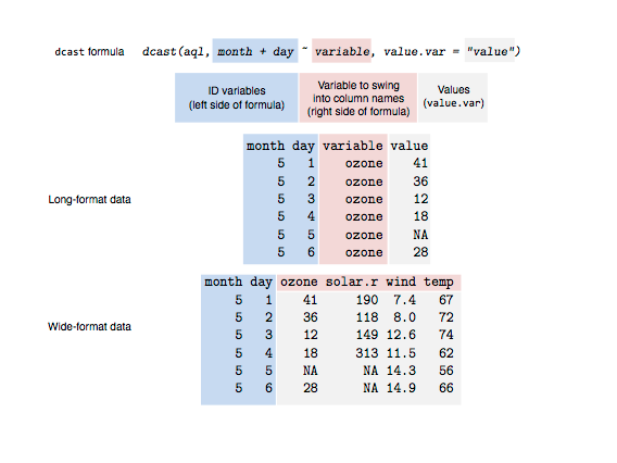
There is a base R dcast() function that is less powerful and slower than the dcast() that comes with data.table. As long as you’ve loaded data.table with library(data.table), you’ll be using the more powerful version of dcast().
- left-side of formula ~: id variables (can be more than 1)
- right-wide of formula ~: columns/variables to split by (can be more than 1)
- value.var: which column has the values (can be more than 1)
dcast(long, student ~ class, value.var = "grades")
  student englishGrades mathGrades physicsGrades
1    Andy             1         10          1000
2    Mary            -2        -20         -2000
wide # compare with dcast() output
# A tibble: 2 x 4
  student englishGrades mathGrades physicsGrades
  <chr>           <dbl>      <dbl>         <dbl>
1 Andy                1         10          1000
2 Mary               -2        -20         -2000
Long to wide with spread() (from tidyverse and tidyr)
spread() is less flexible than dcast()
spread(long, key = class, value = grades)
# A tibble: 2 x 4
  student englishGrades mathGrades physicsGrades
  <chr>           <dbl>      <dbl>         <dbl>
1 Andy                1         10          1000
2 Mary               -2        -20         -2000
wide # compare with spread() output
# A tibble: 2 x 4
  student englishGrades mathGrades physicsGrades
  <chr>           <dbl>      <dbl>         <dbl>
1 Andy                1         10          1000
2 Mary               -2        -20         -2000
Another example
Resources for converting data forms and reshaping
Joining/binding data (rows)
wide # original data
# A tibble: 2 x 4
  student englishGrades mathGrades physicsGrades
  <chr>           <dbl>      <dbl>         <dbl>
1 Andy                1         10          1000
2 Mary               -2        -20         -2000
moreRows <- tibble(student = c("John", "Jane"),
                   englishGrades = c(5, -5),
                   mathGrades = englishGrades * 10,
                   physicsGrades = mathGrades * NA)
moreRows
# A tibble: 2 x 4
  student englishGrades mathGrades physicsGrades
  <chr>           <dbl>      <dbl>         <dbl>
1 John                5         50            NA
2 Jane               -5        -50            NA
rbind(wide, moreRows)
# A tibble: 4 x 4
  student englishGrades mathGrades physicsGrades
  <chr>           <dbl>      <dbl>         <dbl>
1 Andy                1         10          1000
2 Mary               -2        -20         -2000
3 John                5         50            NA
4 Jane               -5        -50            NA
bind_rows(wide, moreRows)
# A tibble: 4 x 4
  student englishGrades mathGrades physicsGrades
  <chr>           <dbl>      <dbl>         <dbl>
1 Andy                1         10          1000
2 Mary               -2        -20         -2000
3 John                5         50            NA
4 Jane               -5        -50            NA
bind_rows has same effect as rbind() above, but much more efficient/flexible and binds even if column numbers don’t match (see below).
moreRows2 <- tibble(student = c("John", "Jane"),
                    englishGrades = c(5, -5),
                    mathGrades = englishGrades * 10)
moreRows2
# A tibble: 2 x 3
  student englishGrades mathGrades
  <chr>           <dbl>      <dbl>
1 John                5         50
2 Jane               -5        -50
wide
# A tibble: 2 x 4
  student englishGrades mathGrades physicsGrades
  <chr>           <dbl>      <dbl>         <dbl>
1 Andy                1         10          1000
2 Mary               -2        -20         -2000
moreRows2 # one less column
# A tibble: 2 x 3
  student englishGrades mathGrades
  <chr>           <dbl>      <dbl>
1 John                5         50
2 Jane               -5        -50
rbind(wide, moreRows2) # error
Error in rbind(deparse.level, ...): numbers of columns of arguments do not match
bind_rows(wide, moreRows2) # no error but fills with NA
# A tibble: 4 x 4
  student englishGrades mathGrades physicsGrades
  <chr>           <dbl>      <dbl>         <dbl>
1 Andy                1         10          1000
2 Mary               -2        -20         -2000
3 John                5         50            NA
4 Jane               -5        -50            NA
Joining/binding data (columns)
Same with rbind(), you can use cbind() to join data by columns. And bind_cols() is much more efficient and flexible.
wide2 <- bind_rows(wide, moreRows2)
wide2
# A tibble: 4 x 4
  student englishGrades mathGrades physicsGrades
  <chr>           <dbl>      <dbl>         <dbl>
1 Andy                1         10          1000
2 Mary               -2        -20         -2000
3 John                5         50            NA
4 Jane               -5        -50            NA
columnsToBind <- tibble(extraCol = c(999, NA, 999, NA))
columnsToBind
# A tibble: 4 x 1
  extraCol
     <dbl>
1      999
2       NA
3      999
4       NA
bind_cols(wide2, columnsToBind)
# A tibble: 4 x 5
  student englishGrades mathGrades physicsGrades extraCol
  <chr>           <dbl>      <dbl>         <dbl>    <dbl>
1 Andy                1         10          1000      999
2 Mary               -2        -20         -2000       NA
3 John                5         50            NA      999
4 Jane               -5        -50            NA       NA
Joining data with left_join() (from tidyverse)
Type ?left_join() in your console to see all other types of joins. I use left_join() most frequently.
Look at the data below. What if we have some information about each student in a separate dataframe and we want to merge the datasets?
wide2
# A tibble: 4 x 4
  student englishGrades mathGrades physicsGrades
  <chr>           <dbl>      <dbl>         <dbl>
1 Andy                1         10          1000
2 Mary               -2        -20         -2000
3 John                5         50            NA
4 Jane               -5        -50            NA
Let’s say we know the gender and chemistry grades of each student…
extraInfo <- tibble(student = c("Jane", "John", "Mary", "Andy"),
                    chemistryGrades = c(900, 901, 902, 903))
extraInfo
# A tibble: 4 x 2
  student chemistryGrades
  <chr>             <dbl>
1 Jane                900
2 John                901
3 Mary                902
4 Andy                903
Can we merge the data wide2 and extraInfo with bind_cols()?
bind_cols(wide2, extraInfo)
# A tibble: 4 x 6
  student...1 englishGrades mathGrades physicsGrades student...5 chemistryGrades
  <chr>               <dbl>      <dbl>         <dbl> <chr>                 <dbl>
1 Andy                    1         10          1000 Jane                    900
2 Mary                   -2        -20         -2000 John                    901
3 John                    5         50            NA Mary                    902
4 Jane                   -5        -50            NA Andy                    903
What’s wrong? How to fix it?
left_join(wide2, extraInfo)
# A tibble: 4 x 5
  student englishGrades mathGrades physicsGrades chemistryGrades
  <chr>           <dbl>      <dbl>         <dbl>           <dbl>
1 Andy                1         10          1000             903
2 Mary               -2        -20         -2000             902
3 John                5         50            NA             901
4 Jane               -5        -50            NA             900
Is the output what you expect? Is it correct? What does the ‘Joining, by = “student”’ mean?
What if we have missing/incomplete extra information?
extraInfo2 <- tibble(student = c("Jane", "John"), chemistryGrades = c(900, 901))
extraInfo2
# A tibble: 2 x 2
  student chemistryGrades
  <chr>             <dbl>
1 Jane                900
2 John                901
left_join(wide2, extraInfo2)
# A tibble: 4 x 5
  student englishGrades mathGrades physicsGrades chemistryGrades
  <chr>           <dbl>      <dbl>         <dbl>           <dbl>
1 Andy                1         10          1000              NA
2 Mary               -2        -20         -2000              NA
3 John                5         50            NA             901
4 Jane               -5        -50            NA             900
Works! Rows with missing information have NA.
Note that you can specify which columns/variables to join by via the by parameter in all join functions. By default, R automatically finds matching column/variable names between both data objects and joins by ALL matching columns/variables.
Also, the output class of join functions are not data.table! To convert class, use pipes!
class(left_join(wide2, extraInfo2)) # not data.table (no...)
[1] "tbl_df" "tbl" "data.frame"
left_join(wide2, extraInfo2) %>% as.data.table() # convert to data.table
   student englishGrades mathGrades physicsGrades chemistryGrades
1:    Andy             1         10          1000              NA
2:    Mary            -2        -20         -2000              NA
3:    John             5         50            NA             901
4:    Jane            -5        -50            NA             900
left_join(wide2, extraInfo2) %>% as.data.table() %>% class() # check class (data.table! yea!)
[1] "data.table" "data.frame"Within-subjects, between-subjects designs, covariates
Create some data
gradesWide <- left_join(wide2, extraInfo2)
gradesWide
# A tibble: 4 x 5
  student englishGrades mathGrades physicsGrades chemistryGrades
  <chr>           <dbl>      <dbl>         <dbl>           <dbl>
1 Andy                1         10          1000              NA
2 Mary               -2        -20         -2000              NA
3 John                5         50            NA             901
4 Jane               -5        -50            NA             900
Wide form data is good for dependent/paired t.tests in R (within-subjects)
t.test(gradesWide$englishGrades, gradesWide$mathGrades, paired = T)
    Paired t-test

data:  gradesWide$englishGrades and gradesWide$mathGrades
t = 0.11704, df = 3, p-value = 0.9142
alternative hypothesis: true difference in means is not equal to 0
95 percent confidence interval:
 -58.92937  63.42937
sample estimates:
mean of the differences
                   2.25
t.test(gradesWide$englishGrades, gradesWide$chemistryGrades, paired = T)
    Paired t-test

data:  gradesWide$englishGrades and gradesWide$chemistryGrades
t = -200.11, df = 1, p-value = 0.003181
alternative hypothesis: true difference in means is not equal to 0
95 percent confidence interval:
 -957.6779 -843.3221
sample estimates:
mean of the differences
                 -900.5
But long-form data is generally preferred
gradesLong <- melt(gradesWide, id.vars = "student", variable.name = "class", value.name = "grade") %>%
    arrange(student) %>% # sort by student
    as.data.table() # convert to data.table and tibble
gradesLong
    student           class grade
 1:    Andy   englishGrades     1
 2:    Andy      mathGrades    10
 3:    Andy   physicsGrades  1000
 4:    Andy chemistryGrades    NA
 5:    Jane   englishGrades    -5
 6:    Jane      mathGrades   -50
 7:    Jane   physicsGrades    NA
 8:    Jane chemistryGrades   900
 9:    John   englishGrades     5
10:    John      mathGrades    50
11:    John   physicsGrades    NA
12:    John chemistryGrades   901
13:    Mary   englishGrades    -2
14:    Mary      mathGrades   -20
15:    Mary   physicsGrades -2000
16:    Mary chemistryGrades    NA
What if we want to use englishGrades as a covariate? Then the covariate has to be in a separate column/variable.
Subset data with just covariate and id variable
covariate_englishGrades <- gradesLong[class == "englishGrades", .(student, grade)]
covariate_englishGrades
   student grade
1:    Andy     1
2:    Jane    -5
3:    John     5
4:    Mary    -2
Rename covariate
setnames(covariate_englishGrades, "grade", "englishGrades")
covariate_englishGrades
   student englishGrades
1:    Andy             1
2:    Jane            -5
3:    John             5
4:    Mary            -2
Use left_join() to add covariate to data
gradesLong_covariate <- left_join(gradesLong, covariate_englishGrades) %>% as.data.table()
gradesLong_covariate
    student           class grade englishGrades
 1:    Andy   englishGrades     1             1
 2:    Andy      mathGrades    10             1
 3:    Andy   physicsGrades  1000             1
 4:    Andy chemistryGrades    NA             1
 5:    Jane   englishGrades    -5            -5
 6:    Jane      mathGrades   -50            -5
 7:    Jane   physicsGrades    NA            -5
 8:    Jane chemistryGrades   900            -5
 9:    John   englishGrades     5             5
10:    John      mathGrades    50             5
11:    John   physicsGrades    NA             5
12:    John chemistryGrades   901             5
13:    Mary   englishGrades    -2            -2
14:    Mary      mathGrades   -20            -2
15:    Mary   physicsGrades -2000            -2
16:    Mary chemistryGrades    NA            -2
# remove englishGrades from long form data if necessary
gradesLong_covariate2 <- gradesLong_covariate[class != "englishGrades"]
gradesLong_covariate2
    student           class grade englishGrades
 1:    Andy      mathGrades    10             1
 2:    Andy   physicsGrades  1000             1
 3:    Andy chemistryGrades    NA             1
 4:    Jane      mathGrades   -50            -5
 5:    Jane   physicsGrades    NA            -5
 6:    Jane chemistryGrades   900            -5
 7:    John      mathGrades    50             5
 8:    John   physicsGrades    NA             5
 9:    John chemistryGrades   901             5
10:    Mary      mathGrades   -20            -2
11:    Mary   physicsGrades -2000            -2
12:    Mary chemistryGrades    NA            -2
Fit model with covariate using lm() (linear model)
summary(lm(grade ~ class + englishGrades, data = gradesLong_covariate2))
Call:
lm(formula = grade ~ class + englishGrades, data = gradesLong_covariate2)

Residuals:
       1        2        4        6        7        9       10       11
  -45.31  1430.63   172.17   230.74  -190.30  -230.74    63.43 -1430.63

Coefficients:
                     Estimate Std. Error t value Pr(>|t|)
(Intercept)             9.062    517.300   0.018    0.987
classphysicsGrades   -485.938    895.308  -0.543    0.616
classchemistryGrades  891.438    895.308   0.996    0.376
englishGrades          46.247     98.870   0.468    0.664

Residual standard error: 1033 on 4 degrees of freedom
  (4 observations deleted due to missingness)
Multiple R-squared:  0.3477,    Adjusted R-squared:  -0.1415
F-statistic: 0.7108 on 3 and 4 DF,  p-value: 0.5943
Get ANOVA output from lm() output
summary.aov(lm(grade ~ class + englishGrades, data = gradesLong_covariate2))
              Df  Sum Sq Mean Sq F value Pr(>F)
class          2 2043615 1021808   0.957  0.458
englishGrades  1  233664  233664   0.219  0.664
Residuals      4 4271812 1067953
4 observations deleted due to missingness
anova(lm(grade ~ class + englishGrades, data = gradesLong_covariate2))
Analysis of Variance Table

Response: grade
              Df  Sum Sq Mean Sq F value Pr(>F)
class          2 2043615 1021808  0.9568 0.4575
englishGrades  1  233664  233664  0.2188 0.6643
Residuals      4 4271812 1067953
Fit model with covariate using aov() (ANOVA)
summary(aov(grade ~ class + englishGrades, data = gradesLong_covariate2))
              Df  Sum Sq Mean Sq F value Pr(>F)
class          2 2043615 1021808   0.957  0.458
englishGrades  1  233664  233664   0.219  0.664
Residuals      4 4271812 1067953
4 observations deleted due to missingness