Data science: Programming and data science basics

Get source code for this RMarkdown script here.

Consider being a patron and supporting my work?

Donate and become a patron: If you find value in what I do and have learned something from my site, please consider becoming a patron. It takes me many hours to research, learn, and put together tutorials. Your support really matters.

What is data science?

Cleaning, wrangling, and munging data
Summarizing and visualizing data
Fitting models to data
Evaluating fitted models

Setting up: Installing R packages/libraries `install.packages()`

Use the install.packages() function to install packages from CRAN (The Comprehensive R Archive Network), which hosts official releases of different packages (also known as libraries) written by R users (people like you and I can write these packages). For more info, see this tutorial on installation.

Install packages all at once, calling install.packages() function just once, using the c() (combine/concatenate) to combine all your package names into one big vector (more on what vectors and classes are later).

Install packages once and you’ll have them on your computer. You only need to update them regularly in the future. No need to rerun install.packages() every time you want to use these packages.


install.packages(c("data.table", "tidyverse"))

Using/loading R packages when you begin a new RStudio session `library()`

Use library() to load packages and use semi-colon (;) to load multiple packages in the same line. I always load the packages below whenever I start a new RStudio session. Sometimes you’ll see people using require() instead of library(). Both works!


library(data.table); library(tidyverse)

Changing R default option settings

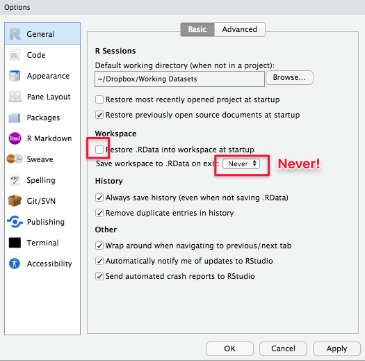
I also strongly recommend changing a few default R options. Click on RStudio -> Preferences -> General Tab and (un)check the boxes below.

You might want to change your default working directory at the top (mine is ~Dropbox/Working Datasets). This directory will be where RStudio saves all your work automatically if you don’t manually specify/change your working directory later on (more on directories later on).
By default, RStudio reloads your previously saved work whenever you reopen it, which can often be disastrous (just like you might not want Microsoft Word to always reopen the document you last worked on every single time you open it). So we are disabling (unchecking) relevant features (uncheck the highlighted box below and select Never).

Working/current directory: Where are you and where should you be? `getwd()`

The working directory (also known as current directory) is the folder (also known as directory) you’re currently in. If you’re navigating your computer with your mouse, you’ll be clicking and moving into different folders. Directory is just a different way of saying ‘location’ or where you’re at right now (which folder you’re currently in).


getwd() # prints in the console your current directory


[1] "/Users/hause/Dropbox/Working Projects/R_websites/rtutorials"

The path above tells you where your working directory is now. It’s conceptually equivalent to you opening a window and using your mouse to manually navigate to that folder.

The [1] in the output refers to the element number of your output.

To change your working directory (to where your project folder is located), use the setwd(). This function is easy to use, but the difficulty for most beginners is getting the path to your folder (e.g., "/Users/Hause/Dropbox/Working Projects/RDataScience") so you can specify something like setwd("/Users/Hause/Dropbox/Working Projects/RDataScience").

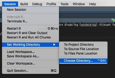
Two ways to change/set your working directory (both uses `setwd()`).

Go to your menubar (at the top). Click Help and search for set working directory. RStudio will tell you how to do it via the Session menu. Select Set Working Directory and Choose Directory. Then navigate to your project directory and you’re done.

On one of the RStudio panes, you’ll see a Files tab (click on it). Use that pane to navigate to your project directory. When you’re there, click More and Set As Working Directory.

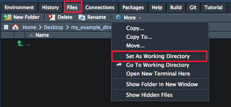
Whether you choose method 1 or 2, you should see your new directory being set in the console panel, which should look something like > setwd("your/path/is/here"). COPY AND PASTE THIS OUTPUT (but without the >) to your current script. So you should be copying something like this:


setwd("your/path/is/here")

Getting help via ? or `help()`

To get help and read the documentation for any function, use ? or the help() function. Equivalent ways to get help:


# get help for mean function
help(mean)
?mean # also works
?mean() # also works

# 3 ways to get help for setwd function
?setwd
?setwd()
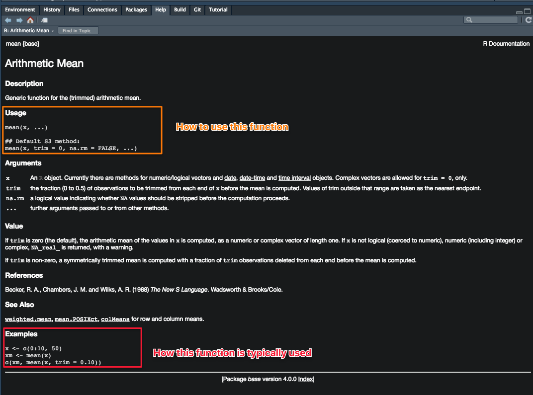
help(setwd)

Beginners will often find the Examples section of the documentation (at the bottom of the document) most useful. Try copying and pasting the code from that section into your script to see how that function works.

Which package does a function come from?

If you ask for help using ? or help(), at the top left corner of the documentation, you’ll see something that looks like functionName{anotherName}, the name within the {} tells you which package a particular function comes from.


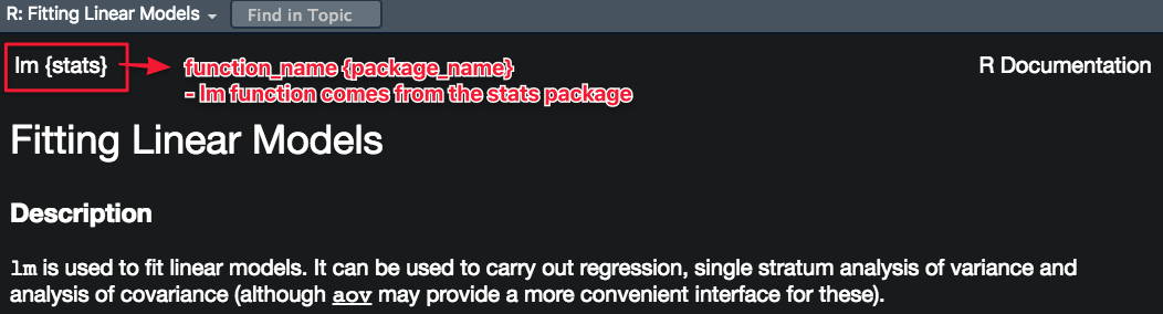
?lm # linear regression, lm{stats} (comes from stats package, which comes with R)
?mean # mean, mean{base} (comes from base package, which comes with R)

To explicitly specify which package to use, you use the following syntax: package::function. Usually we don’t need to explicitly specify which package unless different packages have functions with the same names.


mean(c(1, 2, 3)) # compute mean


[1] 2


base::mean(c(1, 2, 3)) # same as above (explicitly specifies the base package)


[1] 2


# fit linear model/regression function lm(y ~ x, data) (built-in dataset mtcars)
lm(mpg ~ cyl, data = mtcars)


Call:
lm(formula = mpg ~ cyl, data = mtcars)

Coefficients:
(Intercept)          cyl  
     37.885       -2.876


stats::lm(mpg ~ cyl, data = mtcars) # (explicitly specifies the stats package)


Call:
stats::lm(formula = mpg ~ cyl, data = mtcars)

Coefficients:
(Intercept)          cyl  
     37.885       -2.876

Objects, variables, and classes

Objects are ‘things’ in your environment. Just like physical objects (e.g., jeans, frying pan) in your physical environment.

Different objects have different properties, and thus belong to different categories/classes: Jeans belong to clothes and frying pan belongs to utensils. Same with programming language objects: different objects in your environment belong to different categories/classes (often also known as type).

Different categories/classes have different properties and actions associated with them. You wear your jeans but not your frying pan; you can fry eggs with your pan but not your jeans. Same with different programming objects, which includes vectors, lists, dataframes, datatables, matrices, characters (also known as strings), numerics, integers, booleans (and the list goes on).

Different programming objects/classes/categories have different properties and actions associated with them, just like things in everyday life. Birds have wings (a property/feature) and can fly (an action).

You can check the class/category/type of an object with the class() function.


class(mean)


[1] "function"

Note (courtesy of John Eusebio): You can fry your jeans on your frying pan. It’s just not recommended. Same thing with some R functions. You can do some things, like use a for loop to iterate through and operate on every element of a matrix, but you shouldn’t. There are tools that are made to do stuff like matrix operations much more efficiently and effectively.

Creating objects (specifically vectors) with the <- assignment operator

Keyboard shortcut for <- is Alt -


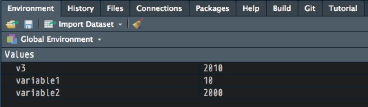
variable1 <- 10 # assign/store the value 10 in variable1
variable2 <- 2000
v3 <- variable1 + variable2 # add variable1 to variable2
variable1; variable2; # print variables to console


[1] 10


[1] 2000


v3 # print variables to console


[1] 2010


print(v3) # same as above v3 (print explicitly prints output to console)


[1] 2010

Check your panes and click on the Environment tab. What do you see there right now? What’s new?

Creating new variables in the environment

Note that R variable names can only begin with characters/letters, not numbers or other symbols.


class(variable1)


[1] "numeric"


class(variable2)


[1] "numeric"


class(v3)


[1] "numeric"


v4 <- c(1, 2, 3, 4, 5) # 'c' stands for concatenate or combine
v4 # prints v4, which is a vector


[1] 1 2 3 4 5

What does c() do?

Vectors are objects that store data of the same class

c() combines values of the same class into a vector (or list).

v4


[1] 1 2 3 4 5


class(v4)


[1] "numeric"


roomsInHouse <- c("Kitchen", "Bedroom") # a vector with all characters
roomsInHouse


[1] "Kitchen" "Bedroom"

Note that all the values in roomsInHouse are in quotation marks "", meaning that the values are all characters (a category or class of objects in R).


class("Date of Birth")


[1] "character"


class(12121999)


[1] "numeric"


mixedClasses <- c("Date of Birth", 12121999)
mixedClasses # what class is this? why?


[1] "Date of Birth" "12121999"


class(mixedClasses)


[1] "character"

Why is it character?


sleep # dataframe that is built into R (comes with any R installation)


   extra group ID
1    0.7     1  1
2   -1.6     1  2
3   -0.2     1  3
4   -1.2     1  4
5   -0.1     1  5
6    3.4     1  6
7    3.7     1  7
8    0.8     1  8
9    0.0     1  9
10   2.0     1 10
11   1.9     2  1
12   0.8     2  2
13   1.1     2  3
14   0.1     2  4
15  -0.1     2  5
16   4.4     2  6
17   5.5     2  7
18   1.6     2  8
19   4.6     2  9
20   3.4     2 10


# for more datasets that came with R, type data()


class(sleep)


[1] "data.frame"

Booleans (class called “logical”): TRUE or FALSE values. TRUE is actually coded as 1 and FALSE coded as 0. Must be all upper-case (TRUE, T, FALSE, F). Lower-case doesn’t work!


booleanExample <- c(T, F)
class(booleanExample) # true


[1] "logical"


class(c(TRUE, FALSE))


[1] "logical"


class(F) # false


[1] "logical"


class(c(T, F))


[1] "logical"

Side note: variable naming conventions

Also, you can use different variable naming conventions. I use both the snake case and camel case (just two of the many conventions).

snake case: my_variable, rooms_in_house, model_output (looks like a snake)
camel case: myVariable, roomsInHouse, modelOutput (looks like a camel)

Indices and indexing with [i, j]

	Column 1	Column 2	Column 3
Row 1	i = 1, j = 1	i = 1, j = 2	i = 1, j = 3
Row 2	i = 2, j = 1	i = 2, j = 2	i = 2, j = 3
Row 3	i = 3, j = 1	i = 3, j = 2	i = 3, j = 3

i: row index, j: column index

Index is just a fancy way of saying numbering or counting. R begins counting from 1 (i.e., indexing begins from 1), whereas many other languages like Python and JavaScript begin from 0.


# create a matrix with values 10, 20, 30, 40, and make it 2 rows long
example_matrix <- matrix(c(10, 20, 30, 40), nrow = 2) 
example_matrix


     [,1] [,2]
[1,]   10   30
[2,]   20   40

To select specific values in the matrix, use the [i, j] syntax, where i refers to the row number and j refers to the column number.


# what does this return? ('return' is a way to say "output" or "spit/print out")
example_matrix[1, 2]


[1] 30

What indices would you use to get the value 20 specifically?


example_matrix[2, 1]


[1] 20

Using functions

Functions take some input, transform that input, and spits out (return is the technical term) some output.


mean(c(10, 20, 30)) # mean function


[1] 20

What is the input to the mean() function above? What is the output?

mean() is the function you call (technical term)
c(10, 20, 30) is the input you provide to the function mean()
the function call mean(c(10, 20, 30)) returns the value 20

In case you’re more familiar with math notation \(y = f(x)\): x is the input to the function \(f()\), and y is the output of the function \(f(x)\).

What are the inputs to the matrix() function below? How is the matrix() function transforming your input? What do you think the output will be?


matrix(c(10, 20, 30, 40, 50, 60), nrow = 6)


     [,1]
[1,]   10
[2,]   20
[3,]   30
[4,]   40
[5,]   50
[6,]   60


matrix(c(10, 20, 30, 40, 50, 60), ncol = 6)


     [,1] [,2] [,3] [,4] [,5] [,6]
[1,]   10   20   30   40   50   60


matrix(c(10, 20, 30, 40, 50, 60), nrow = 2)


     [,1] [,2] [,3]
[1,]   10   30   50
[2,]   20   40   60


matrix(c(10, 20, 30, 40, 50, 60), nrow = 2, byrow = TRUE)


     [,1] [,2] [,3]
[1,]   10   20   30
[2,]   40   50   60


# how does this output differ from the one above?


paste0(c("a", "b", "c"), 1:3) # what is the paste0 function doing?


[1] "a1" "b2" "c3"


paste(c("a", "b", "c"), 1:3) # How is paste() different from paste0() above?


[1] "a 1" "b 2" "c 3"


paste(c("a", "b", "c"), 1:3, sep = '_ _ _') # What's happening?


[1] "a_ _ _1" "b_ _ _2" "c_ _ _3"

Piping or chaining functions with `%>%`

Often we apply multiple functions in succession. We say we wrap or nest functions within functions. Math notation: \(y = h(g(f(x)))\): apply function f to x, then function g to that output, and then function h to that output.


x <- c(10.1, 10.1, 20.3, 20.3, 30.2, 30.7, 30.7)
x


[1] 10.1 10.1 20.3 20.3 30.2 30.7 30.7


mean(x) # mean of values in x


[1] 21.77143


unique(x) # unique values in x


[1] 10.1 20.3 30.2 30.7


mean(unique(x)) # mean of unique values in x


[1] 22.825


round(mean(unique(x))) # round of mean of unique values in x


[1] 23

As you can see, wrapping or nesting functions within functions can be quite difficult to read. We can get rid of such nesting/wrapping with pipes %>%, which is available to you when you load the tidyverse package with library(tidyverse) above. Read %>% as “then”.

Keyboard shortcut for %>%: Shift-Command-M (Mac) or Shift-Ctrl-M (Windows)

Take output of x, then apply unique() to that output.


x %>% unique()


[1] 10.1 20.3 30.2 30.7

Take output of x, then apply unique() to that output, then apply mean() to that output.


x %>% unique() %>% mean()


[1] 22.825

Take output of x, then apply unique() to that output, then apply mean() to that output, then apply round() to that output.


x %>% unique() %>% mean() %>% round()


[1] 23

Same outputs below


round(mean(unique(x))) # less legible


[1] 23


x %>% unique() %>% mean() %>% round() # more legible


[1] 23

Piping with %>% makes it easier to read your code (reading left to right: x %>% unique() %>% mean() %>% round()), rather than from inside to outside: round(mean(unique(x))).

If your pipes get too long, you can separate pipes into different lines.


x %>% # one line at a time (press enter after each pipe)
    unique() %>% 
    mean() %>% 
    round()


[1] 23

In R, this approach of using pipes %>% is called piping. In other languages like Python, it’s called chaining.

Functions and argument order

Make sure to specify your function arguments in the correct order. If not, make sure to specify the name of each argument you’re using!


numbers <- c(1:3, NA)
numbers


[1]  1  2  3 NA

Argument-value pairs: argument is x, value is numbers (defined above as 1, 2, 3, NA)


mean(x = numbers) # what happened?


[1] NA

Argument-value pairs

argument1 = x, value = numbers
argument2 = na.rm, value = TRUE


# remove missing (NA) values by giving the value TRUE to the na.rm argument
mean(x = numbers, na.rm = TRUE)


[1] 2

Reading function documentation

To improve as a programmer, you’ll need to learn to read and understand documentation. R’s documentation is quite intuitive once you understand how to read it.


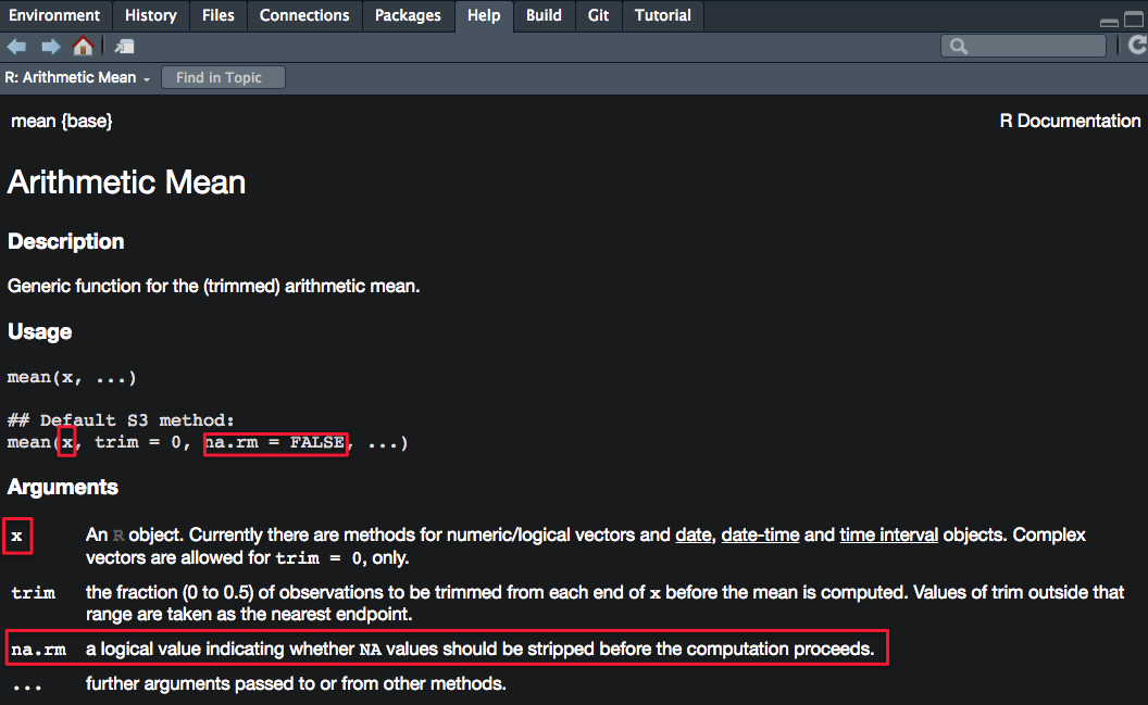
?mean  # show help documentation

Decoding the Usage and Arguments sections

Usage section

mean(x, ...): the function mean() can be called/used by providing one argument (x), which has no default values, so some value/object MUST be provided

mean(x, trim=0, na.rm=FALSE, ...): tells you which arguments have default parameters and what they are (trim parameter has a default value of 0, and na.rm parameter has a default value of FALSE—so NA or missing values are not removed by default); because trim and na.rm have default values, you don’t need to supply them when calling the function mean()

Arguments section

This section provides more details on each parameter of the function.

Note that TRUE can be written simply as T and FALSE can be written as F.


mean(na.rm = T, x = numbers) # does this work?


[1] 2


mean(numbers, na.rm = T) # does this work?


[1] 2


mean(na.rm = T, numbers) # NEVER DO THIS EVEN IF IT WORKS!!! BAD PRACTICE!!!


[1] 2

Why is this so bad?


mean(numbers, TRUE) # what happens? why?


Error in mean.default(numbers, TRUE): 'trim' must be numeric of length one

The function fails to run. Why? Type ?mean in the console and read the documentation to figure out why. What arguments do the mean function also have? What’s the expected order of the arguments?

What are the default values to the arguments? How do you know if there are default values?

Pressing Tab key to autocomplete! Tab will be your best friend!

We often will never remember all the arguments all the functions will require (there are just too many functions!). But when we type the function name followed by brackets mean(), the cursor will automatically move between the brackets. You can press the Tab key on your keyboard to get RStudio to tell you what arguments this function expects.

Be creative! Tab and autocomplete works in MANY other situations! Explore! (variables, filenames, directory paths etc.)

Good practices for reproducible research

One directory/folder per project (create an RProject for each directory/project)
Ensure your working directory is set properly before you begin (use RProjects!)
Ensure your environment is cleared before you begin
Load your libraries at the top of each script
Give your variables and objects sensible names
Optional: save and restore your work with save.image() and load()

Four-step philosophy

Know your subgoals and especially your end goals
Know what you’re passing in to functions
Know what your functions return you
Know how to verify or summarize what your functions return you

Common beginner errors

Not looking at the output in the console (treating R like a black box)
Console still expects more code: + rather than > (press Escape to get rid of +)
Naming your variables un-systematically and calling the wrong variable because of typos
Not knowing what data you’re giving a function
Not knowing what class of data a function expects
Not knowing what class of data your function returns
Not learning how to properly use stackoverflow

Support my work

Support my work and become a patron here!

Programming and data science basics

Table of Contents

Consider being a patron and supporting my work?

What is data science?

Setting up: Installing R packages/libraries `install.packages()`

Using/loading R packages when you begin a new RStudio session `library()`

Changing R default option settings

Working/current directory: Where are you and where should you be? `getwd()`

Two ways to change/set your working directory (both uses `setwd()`).

Getting help via ? or `help()`

Which package does a function come from?

Objects, variables, and classes

Side note: variable naming conventions

Indices and indexing with [i, j]

Using functions

Piping or chaining functions with `%>%`

Functions and argument order

Reading function documentation

Pressing Tab key to autocomplete! Tab will be your best friend!

Good practices for reproducible research

Four-step philosophy

Common beginner errors

Support my work

Corrections

Reuse

Programming and data science basics

Table of Contents

Consider being a patron and supporting my work?

What is data science?

Setting up: Installing R packages/libraries install.packages()

Using/loading R packages when you begin a new RStudio session library()

Changing R default option settings

Working/current directory: Where are you and where should you be? getwd()

Two ways to change/set your working directory (both uses setwd()).

Getting help via ? or help()

Which package does a function come from?

Objects, variables, and classes

Side note: variable naming conventions

Indices and indexing with [i, j]

Using functions

Piping or chaining functions with %>%

Functions and argument order

Reading function documentation

Pressing Tab key to autocomplete! Tab will be your best friend!

Good practices for reproducible research

Four-step philosophy

Common beginner errors

Support my work

Corrections

Reuse

Setting up: Installing R packages/libraries `install.packages()`

Using/loading R packages when you begin a new RStudio session `library()`

Working/current directory: Where are you and where should you be? `getwd()`

Two ways to change/set your working directory (both uses `setwd()`).

Getting help via ? or `help()`

Piping or chaining functions with `%>%`